
Spreadsheets Explained! 5 Levels of Difficulty: From Basic Text Input to Google Apps Script
Five increasingly difficult ways of explaining spreadsheets in Google Sheets: The basics of Google Sheets text Menu items in Google Sheets Math inside Google Sheets Using Formulas in Google Sheets Apps Script in Google Sheets

If you don't think spreadsheets are complicated and complex, then you might not be using them correctly. Or rather, you might not be unleashing all of the power of spreadsheets if you still think that spreadsheets are merely just cells that you put information into. You might not be using the entire power of spreadsheets.
In this tutorial, I’ll walk through five different ways to explain spreadsheets: from almost nothing to the most complex thing, which is Apps Script. Come with me and enjoy this ride!
Five increasingly difficult ways of explaining spreadsheets in Google Sheets:
- The basics of Google Sheets and text
- Menu items in Google Sheets
- Math inside Google Sheets
- Using Formulas in Google Sheets
- Apps Script in Google Sheets
The Basics of Google Sheets Text
First level: The basics of Google Sheets
A spreadsheet is a series of rows and columns that are named by their row number and their column name, which is A, B, C, D. These are still also column 1, column 2, and you can put text into any cell by double clicking on it.
A relation between everything
In Google Sheets, you have a relation between everything on a row and everything in a column.
You can move the entire column over or move an entire row by clicking and dragging on that row.
Here are some things you get to do in Google Sheets:
• Put some text
• Copy and paste text anywhere
• Move the entire column over
• Move an entire row
• Create tables with text
• You can have a header
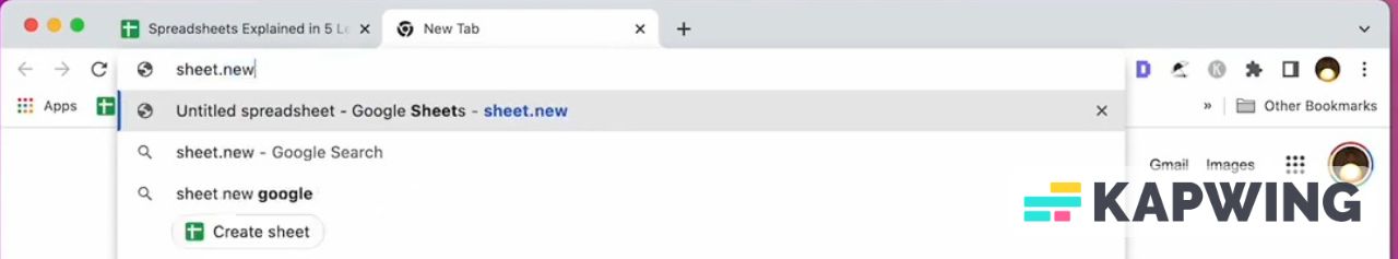
What's interesting about a spreadsheet from Google Sheets is that you can create one by just going to sheet.new and then you create a brand new spreadsheet that's blank, has one tab, 1000 rows, and 26 columns.
Now back to our table.
You can put some text in there and you’ll see their relation.
If we put text in cell A3, you’ll see that our relation of the first one are the texts below it.
Same goes for the second and the third.
The text can go beyond just words. You can also put in numbers and you can format these numbers, which brings us to our next level.
Menu items in Google Sheets
Second level: Menu items
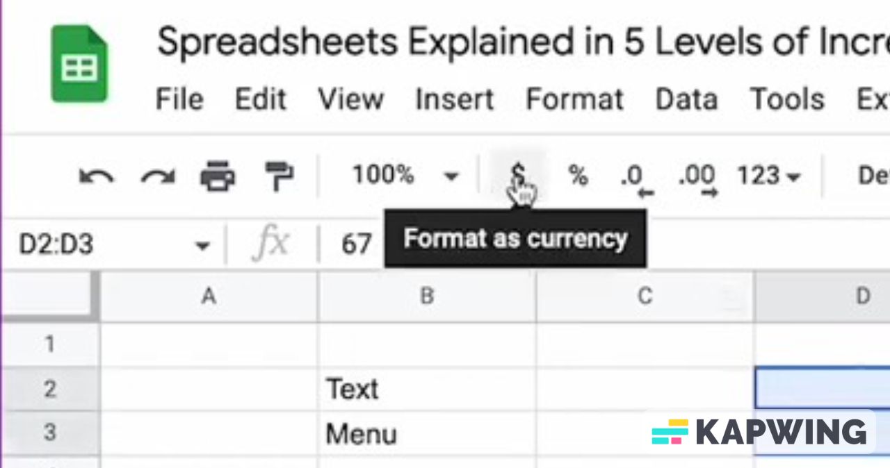
So as you start to create some tables and you put in numbers, such as 67 or 28. And maybe you want to turn these into revenues or money.
What you do is select “Format as currency” in the menu above, where there’s a row of different options.
There are more options for you in the menu above. In these quick select buttons, you can change the text from default Arial to maybe Black Han Sans. You can also change the size of the text. Let’s triple that to 30.
Now you see we have hard to read text here. Let’s make the row bigger. Right click on that row and resize it to a specific number. Instead of fitting to data, we can make this 100 pixels.
If you want to resize more than one row, simply select a row, click the shift button or hold it down. Then we can resize both of those rows at the same time. Let’s give them both a pixel height of 100.
We can do the same with columns. Do right click, shift, and select. Then hit right click and select “Resize columns.” We can resize them to any column size we want.
We can also double click on the gap between rows and it'll automatically resize the row height to the data that you already have in there. If you have nothing inside of the row or column, it will do nothing. But if we have one and two here, you double click and it goes to the minimum size that it can be.
Our menu items also allow us to do alignment of text inside of cells. We can also do wrapping if you get too much text inside of a cell. You can also rotate up and down, and other different directions.
All of these amazing menu items are available to you with just a few clicks. Pretty cool, right?
Math inside spreadsheets
Third level: Math inside of spreadsheets
Just double click on a cell. Start with this format:
=1+0You can try it with the other cells, but this time with different numbers.
=1+1
=1+2
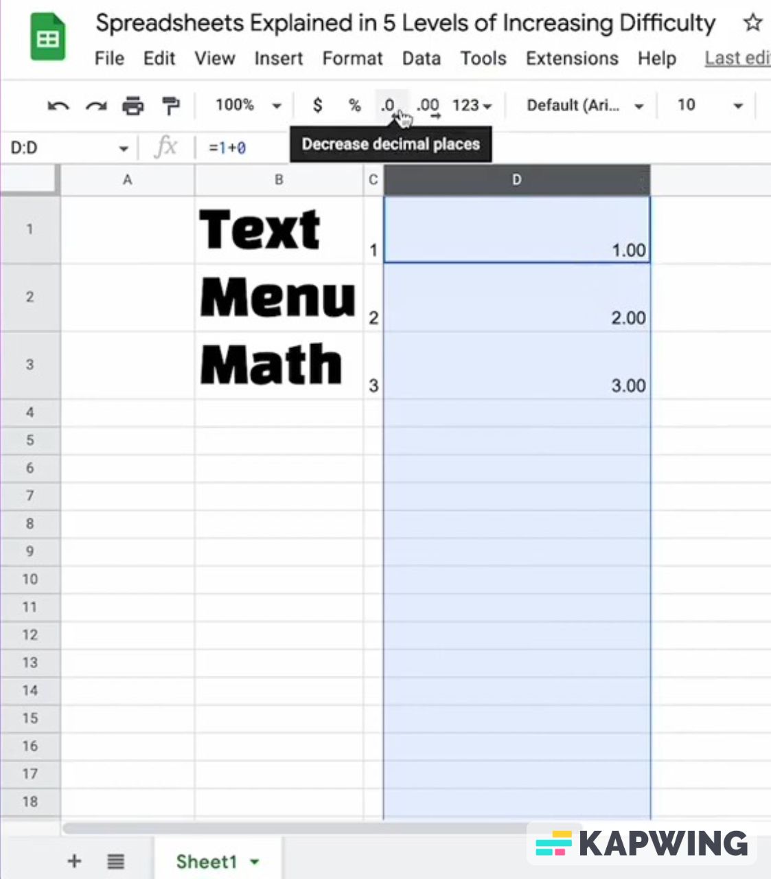
You’ll notice the cells are already pre-formatted. It’s because the format stayed the same from our previous format. We can still change the format back to plain text or a number, which adds 0.00 to it.
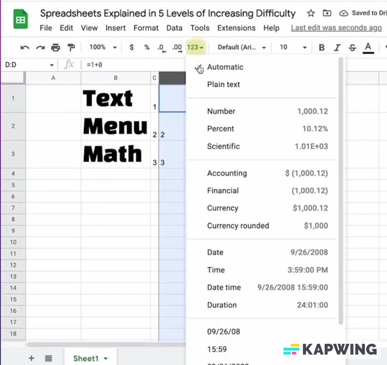
Again, our menu helps us here where we can decrease our decimal place.
You can do all sorts of math in here, such as multiplication. Simply use the asterisk.
=5*5Here’s another cool one: 5 to the power of 5, which would look like this:
=5^5We can also do math inside of cells with words, but it's not exactly as you think. Not with the plus sign. We can say something like "Math is amazing!" with a space here within the quotes in the middle. But the plus sign is not going to work. We need to use an “and” symbol or the ampersand.
Using Formulas in Google Sheets
Fourth level: Math in spreadsheets – Referencing other cells
Are you ready to do something even cooler with Google Sheets? Here it goes...
The most interesting thing with spreadsheets and the power of spreadsheets in math is that we can reference other cells. Instead of typing the word “math”, I can delete that and type in B3 instead. B3 is reference of the cell that is on the B column and is in the third row. This changes based on what I put in B3. Right now, B3 says “Math” but let me change that to “History.” Then D3, which contains words, automatically updates. Now it says "History is awesome!" And that’s the power of spreadsheets.
What might be difficult is coming up with your own formulas and functions. It’s good to know that Google Sheets has some built in formulas and functions that we can use directly. It is all based on having the equal sign show up.
So instead of having something like this:
=D1+D2+D3We can bring up a formula which allows us to reference single cells or arrays of cells or groups of cells that are either in one column or one row.
We use the colon sign to delineate that it is an array. This way, we added up all the numbers we want.
We can also do many other formulas. In fact, there are over 400 formulas in Google Sheets already pre-created for you! Here’s a list of Google Sheets function lists. These are all of the formulas that are available just by typing in equals and then referencing what the name of the formula is. There's a lot of them.
Here are some of my favorites: Average, minimum, and maximum.
If you know all the formulas and all the functions you've done, all the math, you've done all the menus, you know all the menu options. Then there is one more thing that is available to us and that's Apps Script.
Apps Script in Google Sheets
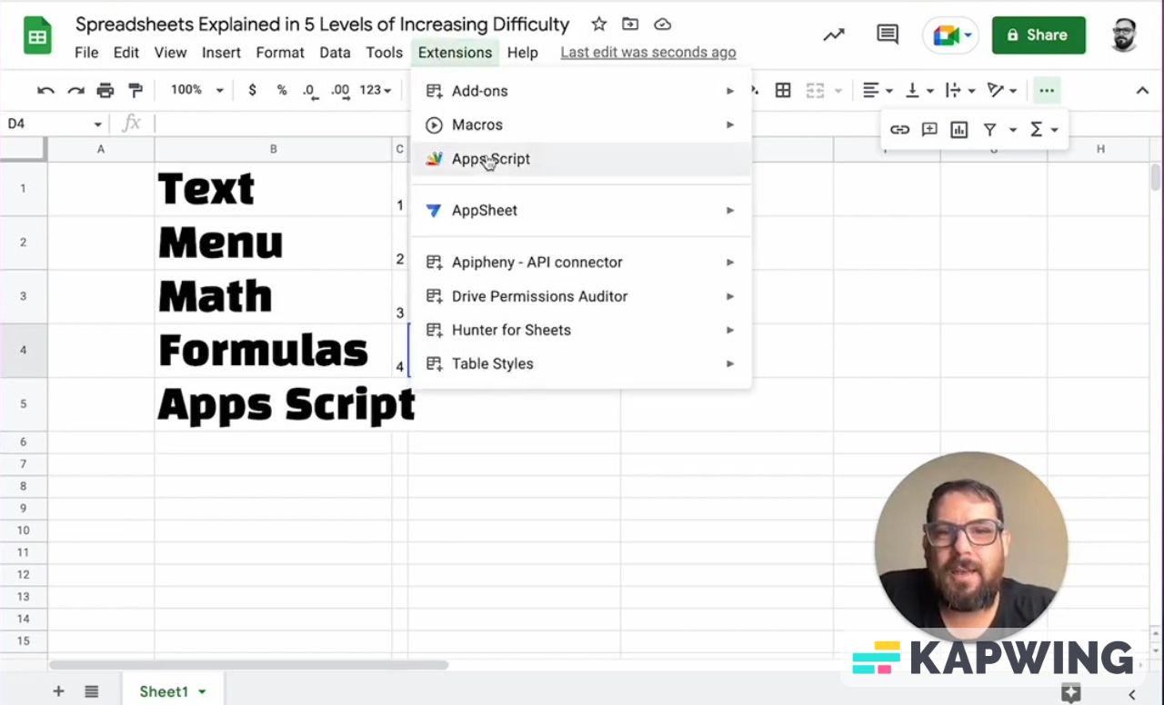
Fifth level: Apps Script in Google Sheets
What is Apps Script?
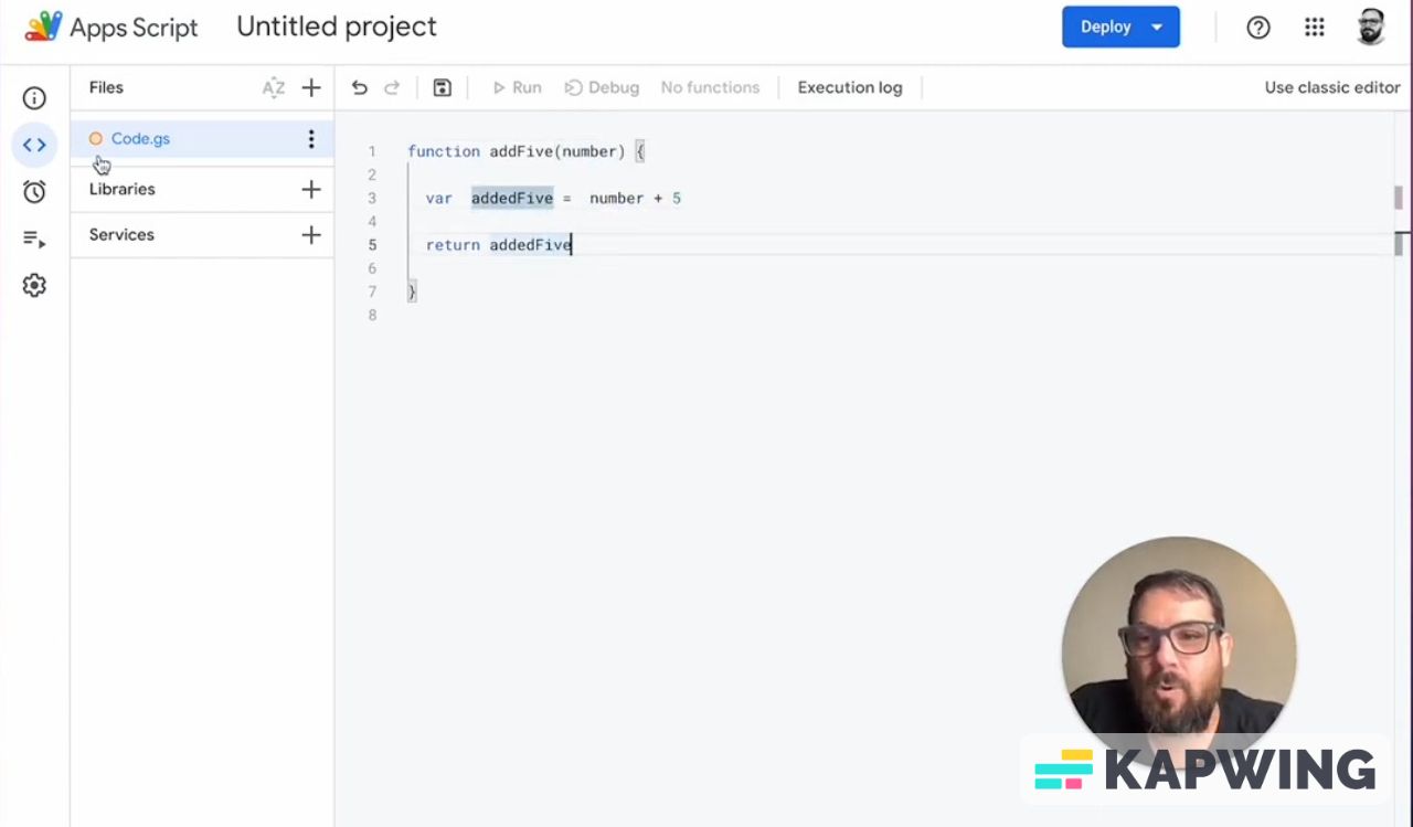
What is Apps Script? It's a handy tool that allows us to create our own custom functions inside of Google. You can access it by going to “Extensions” in the menu and then clicking on Apps Script.
Inside of App Script, we can name and create our very own functions, such as addFive.
In this function we created, we'll take something inside of this parenthesis, like a number.
And in the brackets, we'll do something to it and then we'll return SomethingElse.
We’re going to use variables to do this:
var addedFive = number + 5So here we've taken a variable addedFive.
Then we take the variable number that we put into our formula. We add 5 and then we return addedFive.
Don’t forget to save it! The orange button on the left side tells us we have not saved our project. Let’s hit Command S to save.
So we save our project and now the app script is available to us in our spreadsheet.
Now we can use our function addFive with a number inside of our sheet.
Let’s enter the function we created in a cell. Let’s say we want to add 5 to what’s in C1.
We’ll get a little bit of a red warning here, but we've already created this.
Just hit Enter and there we go.
We get 6!
Now we can copy and paste that same exact formula because we're referencing C1. It's going to change as we copy the function, but it’s still going to keep adding 5 to whatever value is in the cell you entered.
For example: Whatever’s in C2, it adds 5. Whatever’s in C3, it adds 5. This is what the formula we created does.
Now we've created our very own function inside of Google Sheet.
I hope you enjoyed this tutorial. I hope you learned something even deeper about Apps Script and that you'd start to love Google Sheets just like I do.
Don’t make any sheets. Make Better Sheets.
Watch the video for this tutorial:
Watch these tutorials as videos:
Get more Google Sheets Tutorials at BetterSheets.co
Join other members! For $19/month you can access over 200 Better Sheets tutorials. Learn Apps Script in under 40 minutes. Design better dashboards. Make your sheets faster and yourself more confident in sheets.


