So… the other day there was a most interesting discussion over on Twitter/X about the effects of measurement error in linear regression. If you’d like to look at how the discussion went, you can get started here:
Or here, which is where more discussion around the effects of measurement error took place:
I wanted to add my 2 cents to this as well (I mean, I am a psychometrician after all). But the more I thought about it, the more I realized that it would take a lot more than 2 or 3 posts to explain everything I wanted to explain. Which is why I’m writing this in blog format now.
BIG DISCLAIMER: Nothing that I’m about to write down here is new. In fact, this is a combination of my lecture on the effects of measurement error from my Intro to SEM class, as well as (mostly) showcasing examples in R code from the Bollen’s oh-so-classic-of-classics Structural Equations with Latent Variables . More specifically, all of this is taken from Chapter 5: The Consequences of Measurement Error, pp.154 — 167
The model
Bollen does an excellent job at describing exactly what most of us in the social sciences would like to fit as opposed to what we are actually fitting.
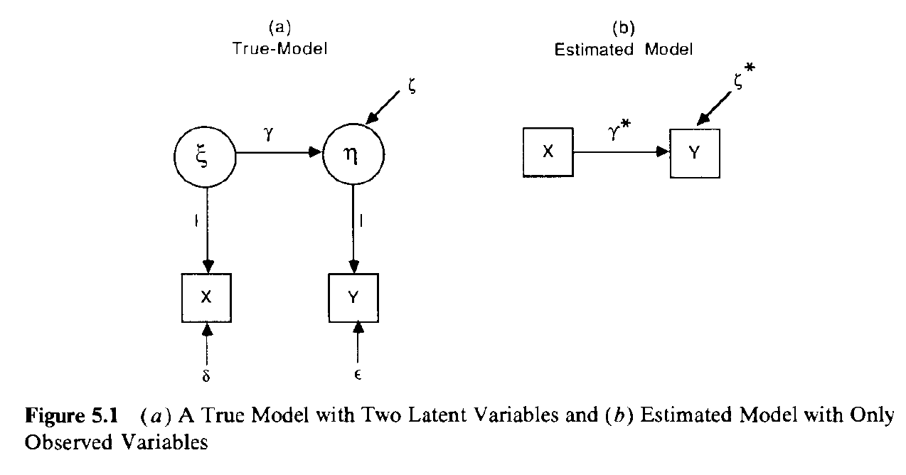
The previous path diagram implies the following system of structural equations:


Covariance and correlation between 

This is the simplest case that I think we’re all familiar with. I’ll reproduce the same results as in Bollen’s Chapter 5, but he makes the assumption that 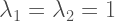


So the covariance of the latent variables is the same as the covariance between the observed values measured with error.
The variance is where things get interesting. Indeed, based on the model above, it follows that:


And since variances are strictly positive, then the following inequality follows trivially:
![\frac{Cov(\xi, \eta)}{\sqrt{[Var(\xi)+Var(\delta)][Var(\eta)+Var(\epsilon)]}} \leq \frac{Cov(\xi, \eta)}{\sqrt{Var(\xi)Var(\eta)}}](https://s0.wp.com/latex.php?latex=%5Cfrac%7BCov%28%5Cxi%2C+%5Ceta%29%7D%7B%5Csqrt%7B%5BVar%28%5Cxi%29%2BVar%28%5Cdelta%29%5D%5BVar%28%5Ceta%29%2BVar%28%5Cepsilon%29%5D%7D%7D+%5Cleq+%5Cfrac%7BCov%28%5Cxi%2C+%5Ceta%29%7D%7B%5Csqrt%7BVar%28%5Cxi%29Var%28%5Ceta%29%7D%7D+&bg=ffffff&fg=444444&s=2&c=20201002)

Simple linear regression between
Although I’m sure some of you are already anticipating what’s going to be in this section, I believe a few of you may be surprised.
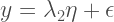
For the simple linear regression model 

But above we derived that

Therefore, we can put it together with the expression for
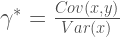
![\gamma^{*}=\gamma \left [ \frac{Var(\xi)}{Var(x)} \right ]](https://s0.wp.com/latex.php?latex=%5Cgamma%5E%7B%2A%7D%3D%5Cgamma+%5Cleft+%5B+%5Cfrac%7BVar%28%5Cxi%29%7D%7BVar%28x%29%7D+%5Cright+%5D+&bg=ffffff&fg=444444&s=2&c=20201002)
So 
So far so good… except there’s a little bit of a “sleight of hand” going on here. Which is the role that 


For a very easy example:

Now, Bollen himself admits that this would be an “unusual situation” (whatever that’s supposed to mean). But, mathematically, it is not impossible. Which means that, in the presence of measurement error, things can increase, decrease or stay the same depending on the measurement model that we are assuming relating the observed and latent variables.
Multiple regression between matrix of predictors 
The much more common case of multiple regression is much more finicky, because we now need to account for the interrelationship of the measurement error across the various predictors. This follows from the identity in Bollen equation (5.25) where he related the matrix of regression coefficients from the latent variables (measured without error) to the matrix of coefficients of te observed variables (measured with error):

So the coefficients of the observed variables, measured with error, are partly a function of the covariance matrix of the predictors themselves (with error) TIMES the covariance between the observed and latent predictors TIMES the matrix of regression coefficients for the latent variables. As I’m sure you can imagine, we’re in an anything goes type scenario, because depending on the 


Bollen presents a very interesting example. Say you’re in a situation with 3 predictors and one dependent variable. But out of the 3 predictors, only 1 of them is measured with error. What would happen to the regression coefficients of the rest of the equation? Now the model (in equation form) looks like this:


Now look at what happens if we plug in some numbers:
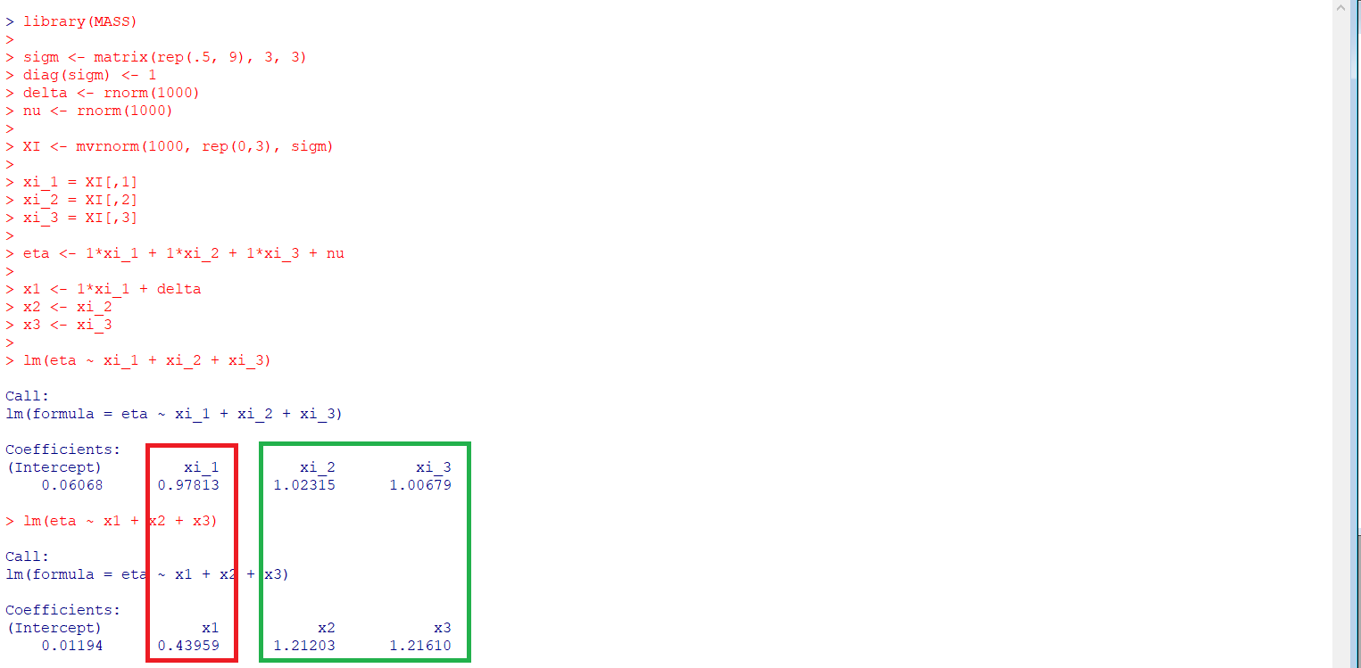
Yes, we see the expected attenuation of the regression coefficient in the presence of measurement error. But look at the effect that that the measurement error in one predictor had in the other predictors, even when measurement error is UNcorrelated ….the coefficients measured without error become inflated. Which is described in equation (5.32) in Bollen:

So the coefficient 


“The direction of asymptotic bias is difficult to predict, since it depends on the magnitude and sign of the second term on the right hand side.“
If you would like to consider a case where all the observed variables have measurement errors with different reliabilities. Look at the following:
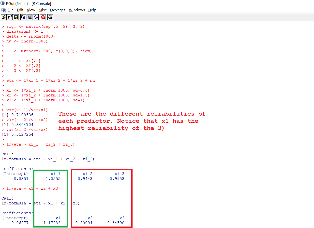
So now the predictor with the highest reliability, 
A lot of our intuitions (and I’m including myself here) regarding the effect that measurement error has on the associations within variables comes mostly from what measurement error does to the variances in a covariance-correlation setting. HOWEVER, without understanding the measurement model that relates the (faulty) observables to the (true) latent variables, we cannot ascertain that the bias for the coefficients will always go down. True, I’m willing to concede that in the majority of cases that we encounter in empirical research, the bias is (i) probably towards 0 more often than not; and (ii) usually, at least one other thing would be biased towards 0. But we need the measurement model to understand where the bias may go.
I’m of the idea that the world we study is infinitely more complicated than what we can imagine. And if we can “imagine” situations where measurement error can bias coefficients upwards as opposed to downwards, I’d say it stands to reason to think that there will be cases in real life where measurement error acts contrary to what our (not-entirely-correct) intuition says.
Anyhoo… my 2 cents ¯\_(ツ)_/¯
