Temporal autocorrelation in GAMs and the mvgam package
By Nicholas Clark in rstats mgcv mvgam
July 16, 2023
Generalized Additive Models (GAMs) are flexible tools that have found particular application in the analysis of time series data. In ecology, a host of recent papers and workshops have drawn attention to the power of GAMs for addressing complex ecological analyses. For example, Gavin Simpson regularly hosts workshops on GAMs in R, and it is common to see GAMs on the workshop list for large international conferences in ecology and statistics.
Why are GAMs useful for time series analysis?
There are several reasons we’d want to use a GAM, particularly one fitted in
the {mgcv} R package, to analyse time series:
- GAMs can be used to model non-linear trends in time series data
- GAMs can easily decompose time series into trend, seasonality and other components
- Smoothing splines can be used to identify periods of rapid historical change
- GAMs can incorporate complex random effects that are common in real time series
Given the many ways that GAMs can model temporal data, it is tempting to extrapolate from their smooth functions to produce out of sample forecasts. Here I inspect how smoothing splines behave when extrapolating outside the training data to examine whether this can be useful in practice. I also discuss some of the pitfalls that tend to arise when trying to fit smoothing splines to temporally autocorrelated data. I then give a few solutions, most notably by making use of Bayesian Dynamic GAMs in the {mvgam} R package.
Environment setup
This tutorial relies on the following packages:
library(mvgam)           # Fit, interrogate and forecast DGAMs
library(dplyr)           # Tidy and flexible data manipulation
library(marginaleffects) # Compute conditional and marginal effects
library(ggplot2)         # Flexible plotting
library(patchwork)       # Combining ggplot objects
First I design a custom ggplot2 theme; feel free to ignore if you have your own plot preferences
theme_set(theme_classic(base_size = 12, base_family = 'serif') +
            theme(axis.line.x.bottom = element_line(colour = "black",
                                                    size = 1),
                  axis.line.y.left = element_line(colour = "black",
                                                  size = 1)))
What are Generalized Additive Models (GAMs)?
The content of this post relates to some concepts I introduced in a recent webinar for the Ecological Forecasting Initiative’s and Ecological Society of America’s Statistical Methods Seminar Series. If you are completely unfamiliar with GAMs, it would be worth a watch to help you catch up on basic concepts.
Wiggliness and autocorrelation
A smoothing spline is composed of basis expansions whose coefficients, which must be estimated, control the functional relationship between a predictor variable and a conditional response. The size of the basis expansion limits the smooth’s potential complexity, with a larger set of basis functions allowing greater flexibility.

All we need to do once we’ve constructed the basis expansion is estimate the weights. This allows us to fit arbitrarily-shaped functions that can learn nonlinear relationships from data

The smoothness of the spline is controlled by a
smoothing penalty, which penalizes functions that are excessively wiggly. The animation below illustrates this process, where the penalty \(\rho\) is chosen to maximise some penalized log(likelihood):

Here I use an exaggerated example to show how a smooth tries to wiggle excessively, leading to overfitting. This can be done by fixing the smoothing penalty \(λ\) in a GAM fit with {mgcv}’s gam() function in R. By fitting models with increasingly relaxed smooths, with \(λ\) values approaching zero, we produce increasingly wiggly fits that tend toward fully unpenalized functions.
par(mfrow = c(2, 2),
    mgp = c(2.5, 1, 0),
    mai=c(c(0.4, 0.7, 0.2, 0.2)))

data(mcycle, package = 'MASS')

m1 <- gam(accel ~ s(times, k = 50),
          data = mcycle, method = 'REML', sp = 5)
plot(m1, scheme = 1, residuals = TRUE, pch = 16,
     bty = 'L',
     ylab = expression(lambda == 5), xlab = '',
     shade.col = scales::alpha("#B97C7C", 0.6))

m2 <- gam(accel ~ s(times, k = 50),
          data = mcycle, method = 'REML', sp = 1)
plot(m2, scheme = 1, residuals = TRUE, pch = 16,
     bty = 'L',
     ylab = expression(lambda == 1), xlab = '',
     shade.col = scales::alpha("#B97C7C", 0.6))

m3 <- gam(accel ~ s(times, k = 50),
          data = mcycle, method = 'REML', sp = 0.01)
plot(m3, scheme = 1, residuals = TRUE, pch = 16,
     bty = 'L',
     ylab = expression(lambda == 0.01), xlab = '',
     shade.col = scales::alpha("#B97C7C", 0.6))

m4 <- gam(accel ~ s(times, k = 50),
          data = mcycle, method = 'REML', sp = 0.0000001)
plot(m4, scheme = 1, residuals = TRUE, pch = 16,
     bty = 'L',
     ylab = expression(lambda == 0.0000001), xlab = '',
     shade.col = scales::alpha("#B97C7C", 0.6))
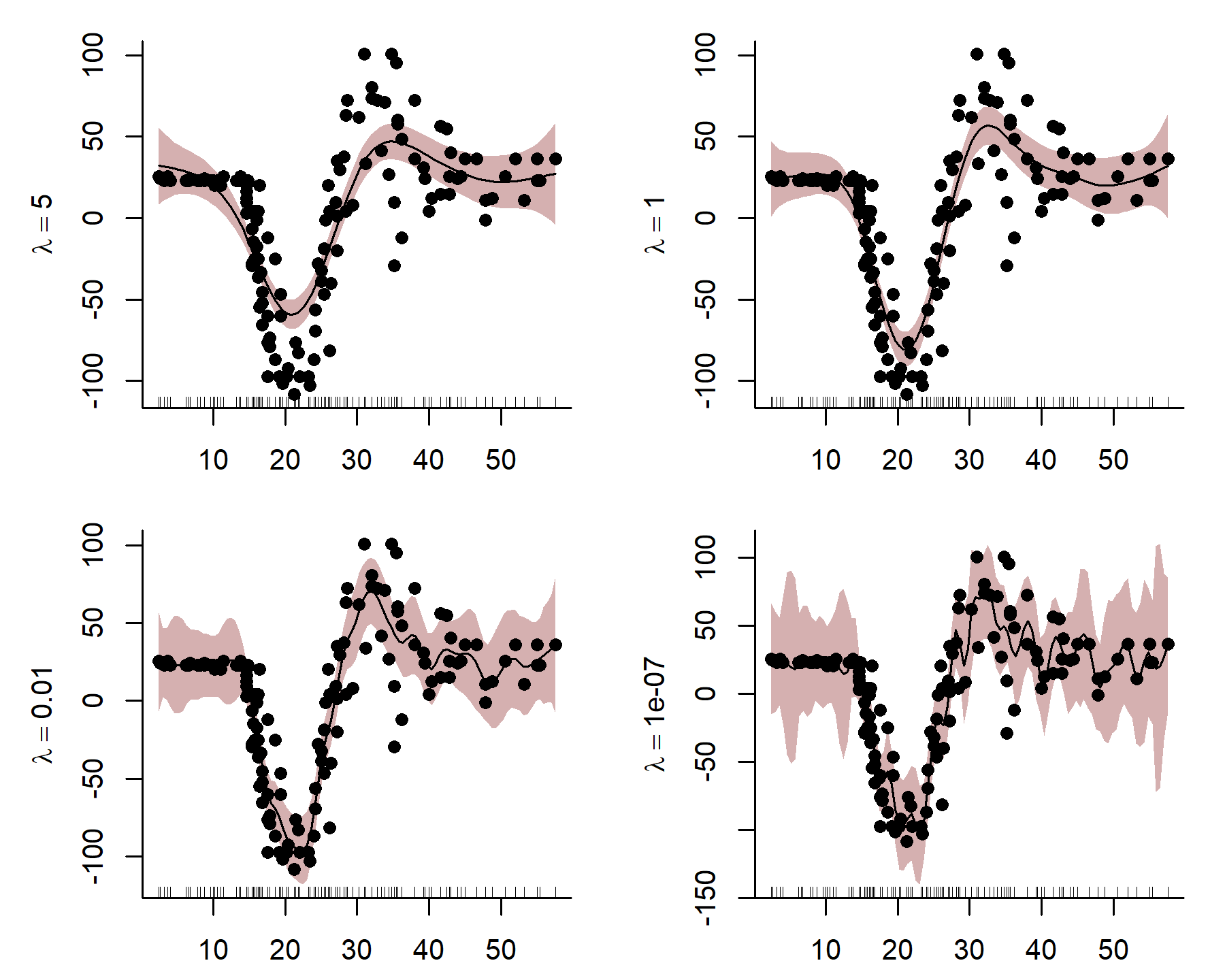
Notice how wiggly the function becomes in the last plot when \(λ\) is very small, indicating that the function is overfitting to the in-sample training data. Incidentally, this behaviour mirrors what often happens when we try to model an autocorrelated time series with a smooth function of time. Unfortunately,
smoothing splines often try to wiggle excessively to capture autocorrelation in a time series. This makes fitting GAMs to time series challenging in some ways. It also leads to poor predictions and forecasts.
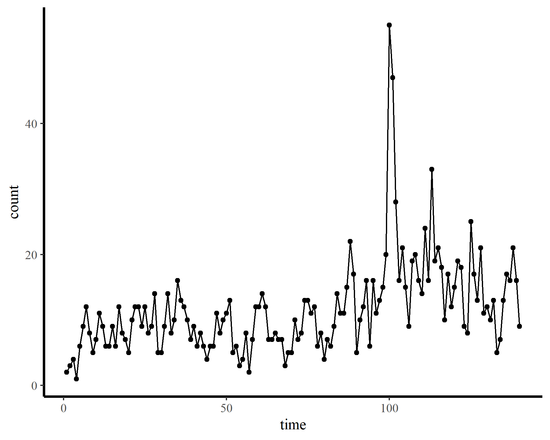
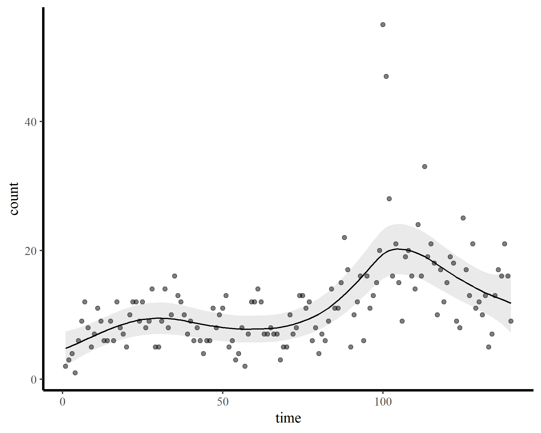
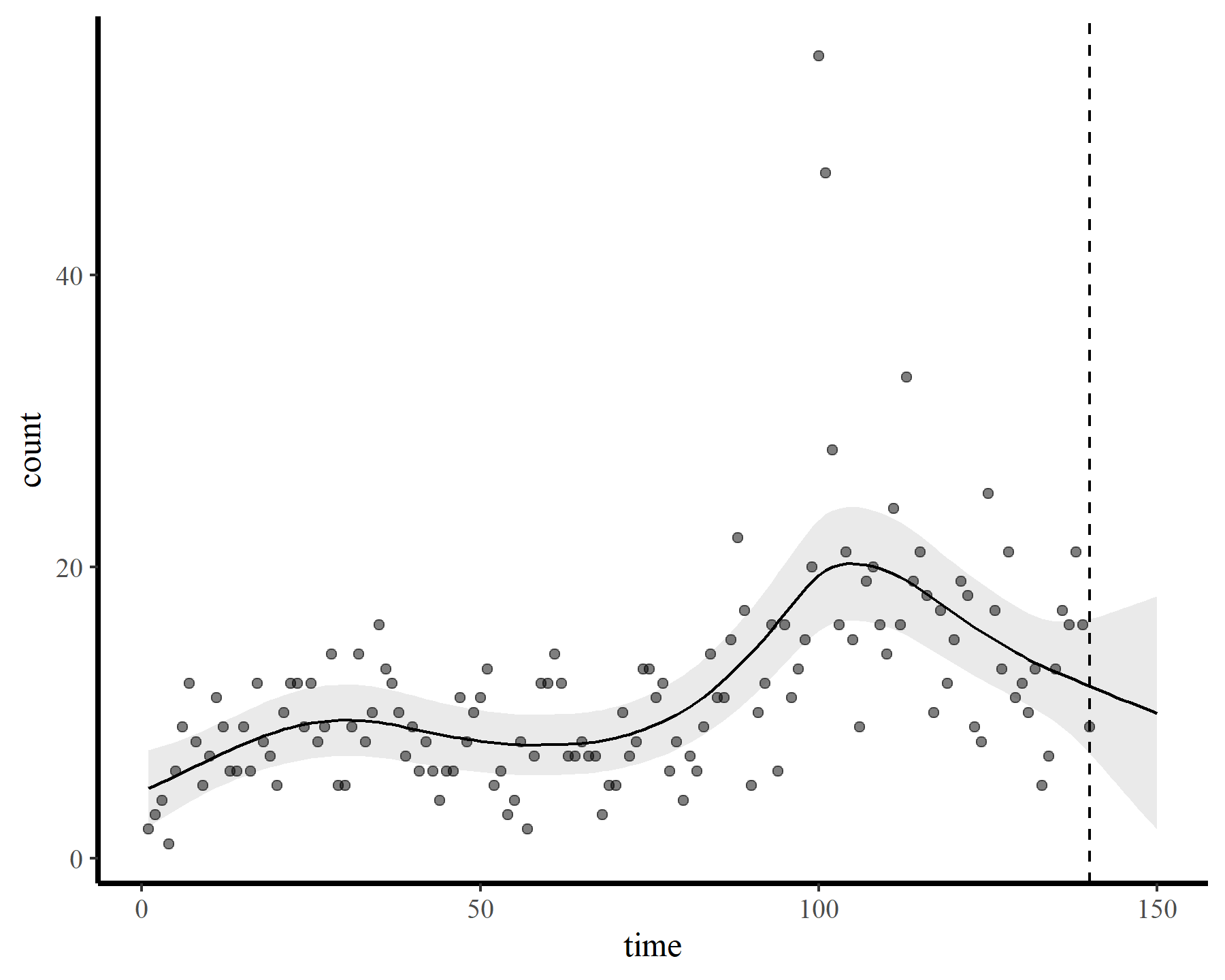
To demonstrate how challenging it can be to work with temporally autocorrelated data in GAMs, I’ll load some time series of counts. The data are from the {tscount} package and represent the umber of campylobacterosis cases (reported every 28 days) in the North of Québec in Canada from January 1990 to the end of October 2000.
# Download the campy data from the tscount package
load(url('https://github.com/cran/tscount/raw/master/data/campy.RData'))

# Put data into a data.frame and visualize
dat <- data.frame(count = as.vector(campy)) %>%
  dplyr::mutate(time = 1:dplyr::n())
ggplot(dat, aes(time, count)) +
  geom_point() +
  geom_line()
Next I supply a few small convenience functions for inspecting model outputs.
# Replicating mgcv::gam.check() but without the plots
small_check = function(model){
  cat("Basis dimension (k) checking results. Low p-value (k-index < 1) may\n")
  cat("indicate that k is too low, especially if edf is close to k\'.\n\n")
  printCoefmat(mgcv::k.check(model), digits = 3)
}

# Call marginaleffects::plot_predictions to inspect model fits
plot_fcs = function(model, n_ahead = 0){
  p <- plot_predictions(model,
                   condition = list(time = 1:(max(dat$time) + n_ahead)),
                   type = 'response',
                   points = 0.5)

  if(n_ahead > 0){
    p <- p +
      geom_vline(xintercept = max(dat$time),
                 linetype = 'dashed')
  }
  p
}

plot_links = function(model, n_ahead = 0){
  p <- plot_predictions(model,
                   condition = list(time = 1:(max(dat$time) + n_ahead)),
                   type = 'link') +
    ylab('linear predictor')

    if(n_ahead > 0){
    p <- p +
      geom_vline(xintercept = max(dat$time),
                 linetype = 'dashed')
  }
  p
}
Now onto some GAMs. My goal is to smooth over the temporal trend in the data and inspect the behaviour of the gam.check() function from {mgcv}. First I impose a restricted smooth of time with a very small number of possible basis functions (using the default thin plate basis). For this and all subsequent models, I stick with a poisson() observation model as this will make it easier to illustrate how the estimated smooth changes as we increase k. After fitting the model, I then check basis dimension and plot the response-scaled predictions
mod1 <- gam(count ~ s(time, k = 6),
            data = dat,
            family = poisson(),
            method = 'REML')
small_check(mod1)
## Basis dimension (k) checking results. Low p-value (k-index < 1) may
## indicate that k is too low, especially if edf is close to k'.
##
##           k'  edf k-index p-value
## s(time) 5.00 4.81    0.61  <2e-16 ***
## ---
## Signif. codes:  0 '***' 0.001 '**' 0.01 '*' 0.05 '.' 0.1 ' ' 1
plot_fcs(mod1)
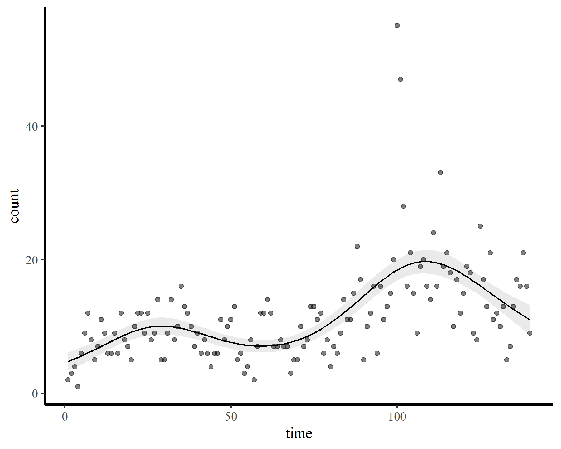
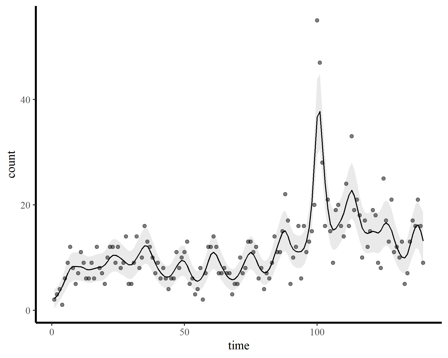
These results strongly indicate that k was set too low (i.e. the k-index is well below 1 and the estimated degrees of freedom is nearly as large as the maximum allowed degrees of freedom). The plot also suggests that the function is not flexible enough to capture the long-term (or short-term) variation in the observed counts. Now for a second model that allows for more possible complexity
mod2 <- gam(count ~ s(time, k = 23),
            data = dat,
            family = poisson(),
            method = 'REML')
small_check(mod2)
## Basis dimension (k) checking results. Low p-value (k-index < 1) may
## indicate that k is too low, especially if edf is close to k'.
##
##           k'  edf k-index p-value
## s(time) 22.0 10.2    0.67  <2e-16 ***
## ---
## Signif. codes:  0 '***' 0.001 '**' 0.01 '*' 0.05 '.' 0.1 ' ' 1
plot_fcs(mod2)
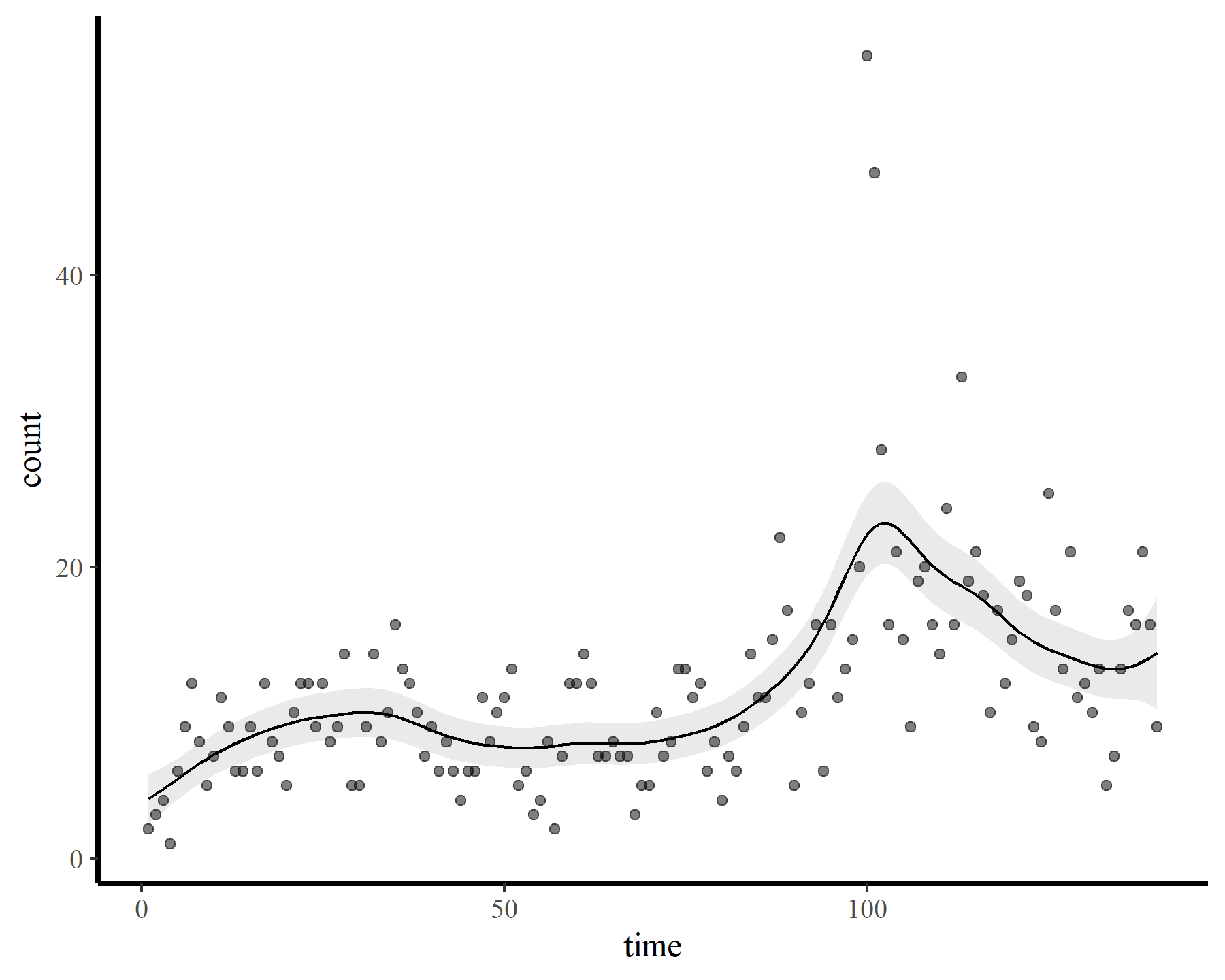
A similar result, with the checking function suggesting that we need to increase k further if we want to capture the patterns that are left in the model residuals. Now for the whole hog, increasing k to the maximum allowed basis dimension
mod3 <- gam(count ~ s(time, k = 140),
            data = dat,
            family = poisson(),
            method = 'REML')
small_check(mod3)
## Basis dimension (k) checking results. Low p-value (k-index < 1) may
## indicate that k is too low, especially if edf is close to k'.
##
##          k' edf k-index p-value
## s(time) 139  31    1.14    0.95
plot_fcs(mod3)
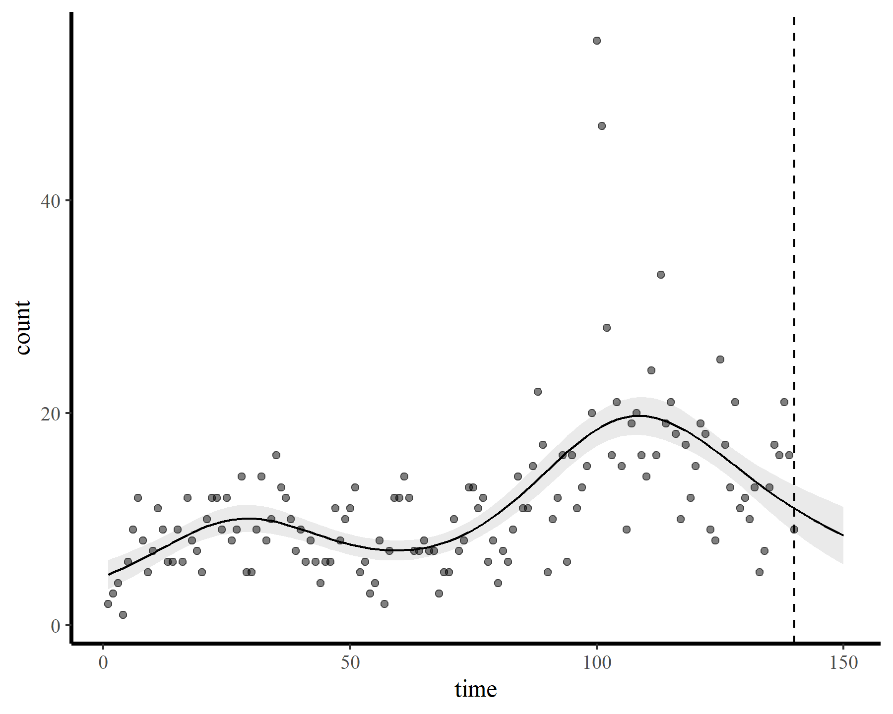
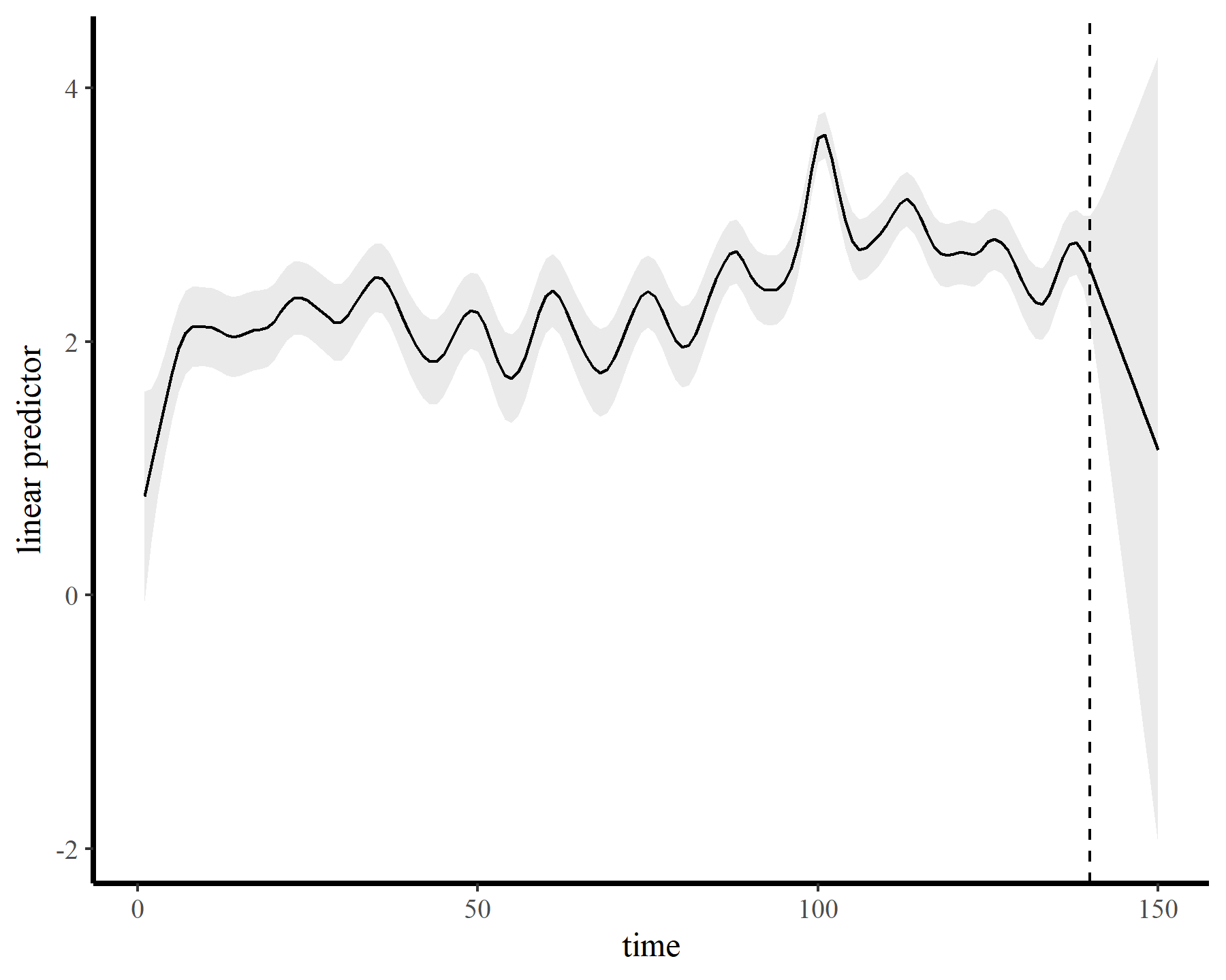
Finally the check suggests the smooth was wiggly enough. But how does this wiggly smooth function behave if we want to extrapolate ahead? Here I predict ahead for 10 timesteps from each of the above models to visualize extrapolation behaviours.
plot_fcs(mod1, 10)
plot_fcs(mod2, 10)
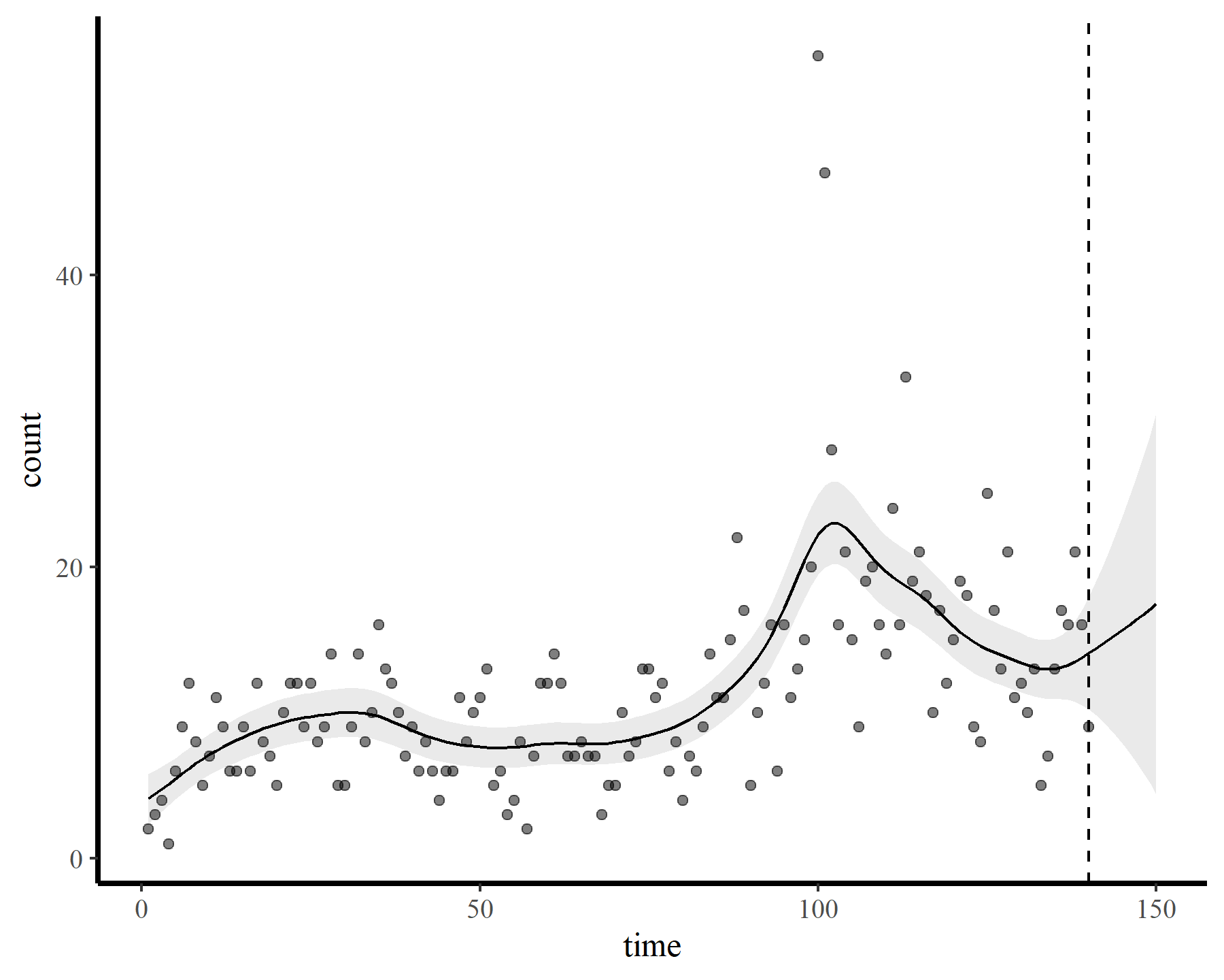
plot_fcs(mod3, 10)
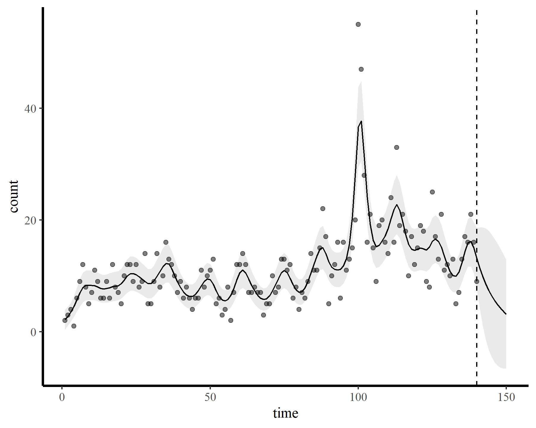
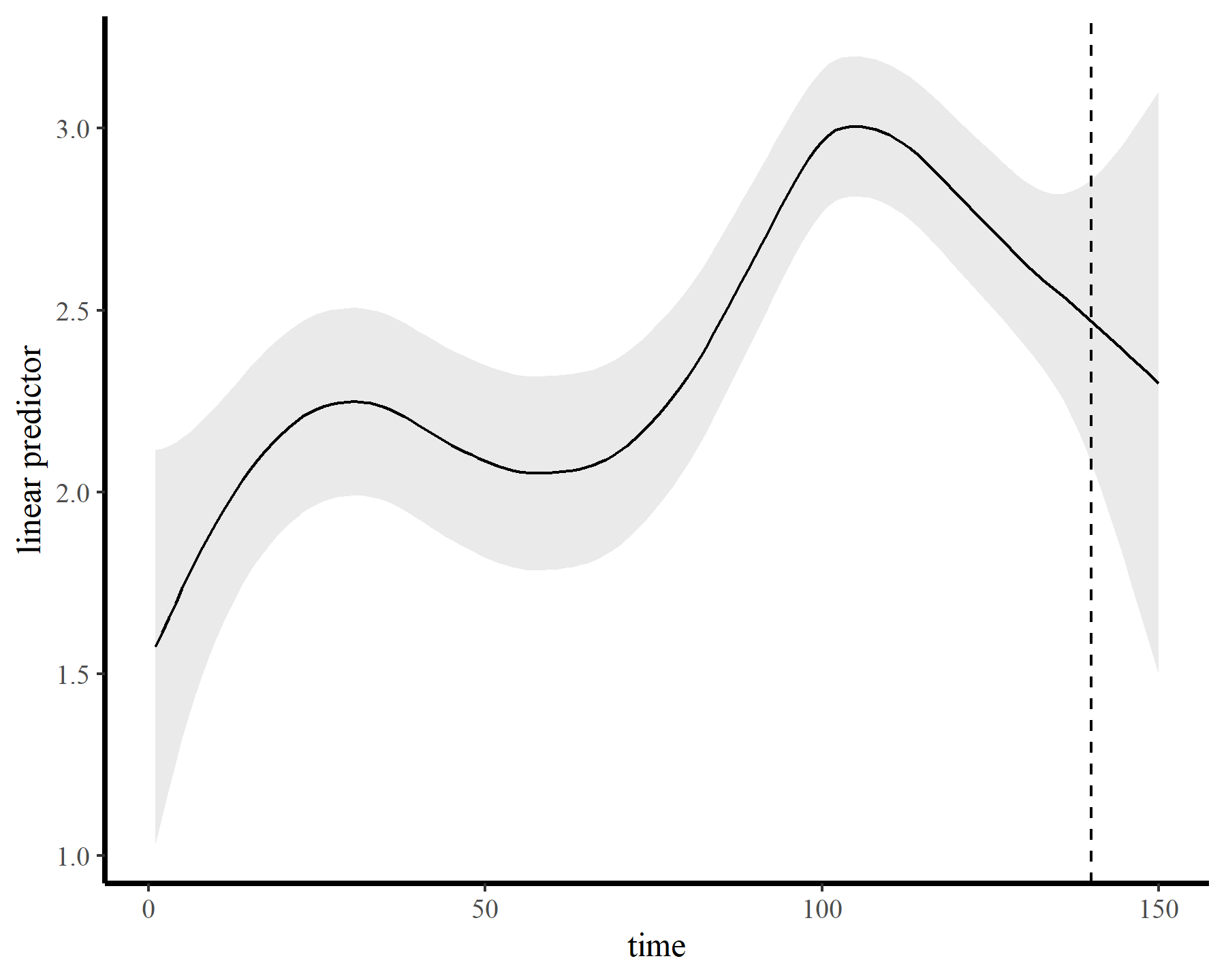
The functions give fairly different forecasts for each model because these penalized splines extrapolate linearly into the future (i.e. if the function wiggled downward toward the end of the training data, the forecast will continue linearly downward forever). This is easier visualized on the link scale
plot_links(mod1, 10)
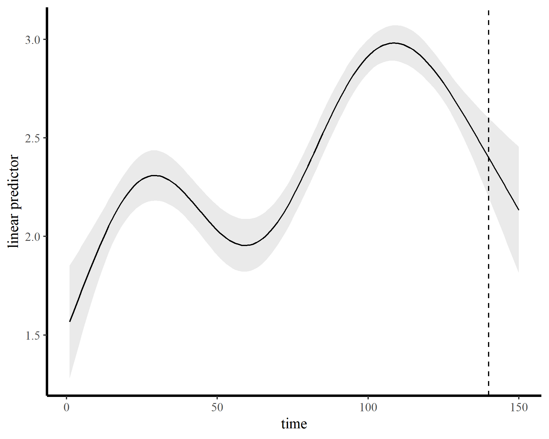
plot_links(mod2, 10)
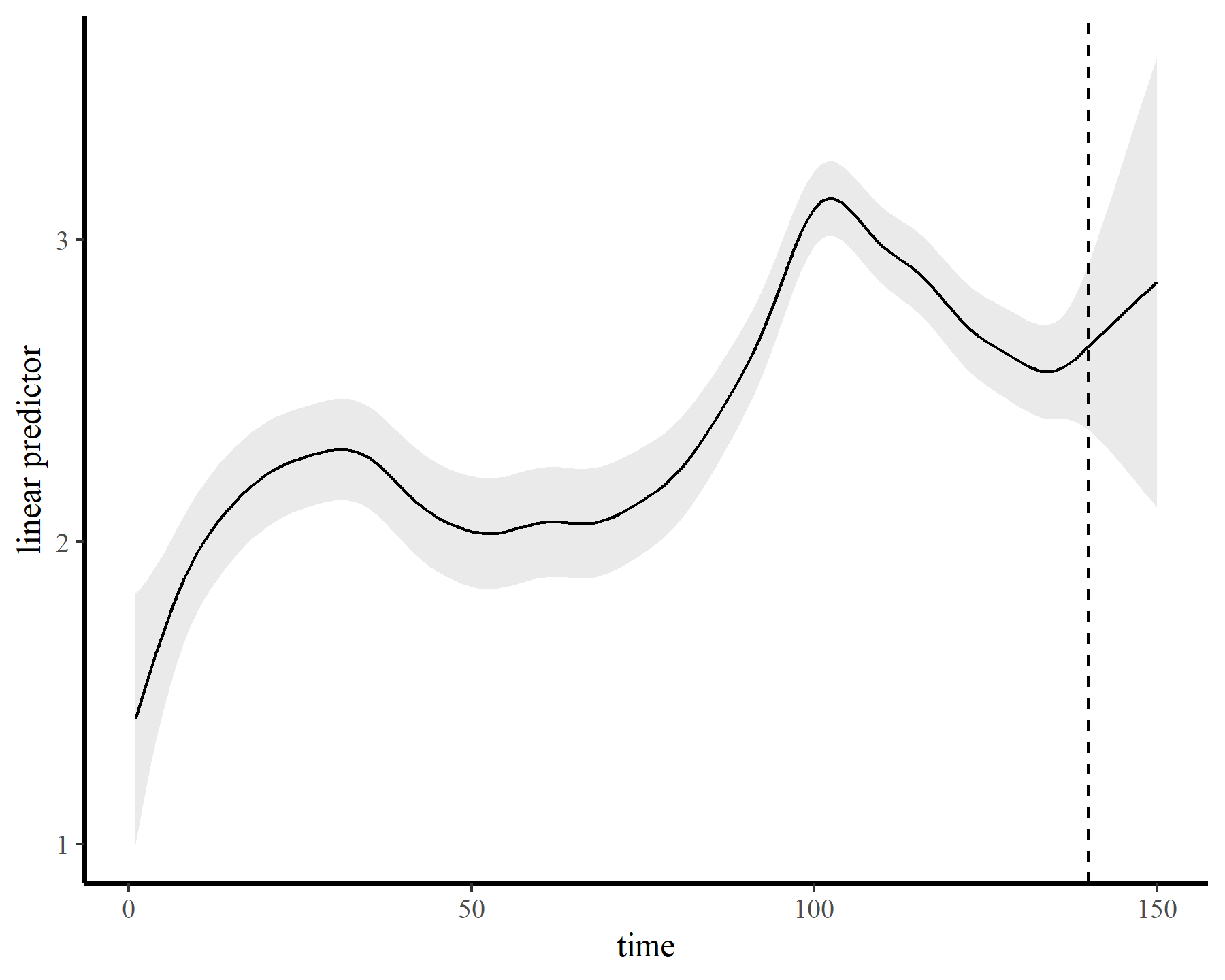
plot_links(mod3, 10)
Autoregressive residuals in mgcv
This behaviour is unwanted, for several reasons. First is the very obvious and unwanted extrapolation behaviour. Not only are these extrapolations typically unrealistic and ignorant of the types of behaviours that occurred within the training data, they are also extremely volatile. Simply by changing k to respect the warnings from gam.check(), we end up with very different ideas about plausible futures. The second reason we don’t want this is that, even if we are not interested in forecasting, chasing autocorrelation with increasingly wiggly smooths increases computational complexity and leads to identifiability issues. Plus there will no doubt be situations in which we cannot capture all of this autocorrelation no matter how wiggly we allow our smooths of time to be.
An obvious solution then is to try and include some sort of residual autocorrelation process in the model. For Gaussian responses, this is fairly straightfoward using the gamm() function, which allows us to supply a correlation argument like those provided by nlme::lme(). We can specify several different forms of stochastic ARMA models that will be used to model the residuals. But we are not using a Gaussian observation model here because our data are non-negative integers. There are other options we can use within gamm() that make use of MASS::glmmPQL() to fit the model, but this can be temperamental and give unsatisfactory results. Finally though, we have the option to use bam() and supply a fixed AR1 coefficient, which will be applied to the working residuals. I’ll illustrate here by fixing the coefficient to 0.6 as a simple example
mod4 <- bam(count ~ s(time, k = 140),
            data = dat,
            family = poisson(),
            rho = 0.6,
            method = 'fREML',
            discrete = TRUE)
small_check(mod4)
## Basis dimension (k) checking results. Low p-value (k-index < 1) may
## indicate that k is too low, especially if edf is close to k'.
##
##             k'    edf k-index p-value
## s(time) 139.00   5.95    0.63  <2e-16 ***
## ---
## Signif. codes:  0 '***' 0.001 '**' 0.01 '*' 0.05 '.' 0.1 ' ' 1
plot_fcs(mod4)
This leads to a much smoother estimate of the smooth, which is good news. We still have the warnings from gam.check() unfortunately, but that is preferable to fitting a smooth that bends all over the place to try and capture the autocorrelation. The extrapolation behaviours are more sensible as well:
plot_fcs(mod4, 10)
plot_links(mod4, 10)
There are still several major downsides to this approach. We have to specify the AR1 coefficient, and if we are modeling several time series in a single joint model (which we very often want to do) we have to use the same AR1 dynamics for each series. We also have no way of incorporating more complex dynamics, such as AR2 or multivariate (VAR) processes. Missing values can cause small or very big problems (the residual AR1 model assumes there is a residual for every timepoint, but if you have missing observations these will be thrown out prior to model fitting). And finally, it is difficult to produce accurate forecasts from this model because our extrapolations do not incorporate the residual autoregressive process. To do so, we’d have to:
- Extract working residuals from the fitted model
- Fit an AR1 model to these residuals using the
fixedargument inarima()to ensure the coefficient is as we specified. This is necessary because we do not know what the variance parameter should be for the residual AR process (it is not returned anywhere in thegamobject - Generate mean expectations (link scale) for the GAM model to cover the out-of-sample validation times
- Predict ahead for the residual AR model to cover the out-of-sample validation times
- Add the two together to generate the linear predictor values, take the inverse link function (using
exp()in this case for the log link) and then use them as the mean values for taking appropriate stochastic draws (usingrpois()in this case)
This process is tedious and error-prone. I won’t work through it here because there is a better way.
Dynamic GAMs using mvgam
The mvgam package was designed to solve these and many other problems we encounter when trying to model realistic time series, produce reliable inferences and generate accurate forecasts. There are many useful vignettes and case studies available (see
documentation on the package website). But I’ll quickly show how we can estimate nonlinear trends and temporal autocorrelation in GAMs. This should allow us to do all the things we want with these models (i.e. calculate rates of change from the trend, interpolate over periods with missing data, produce accurate forecasts). This model uses quite a few of the advanced features of {mvgam}, including:
- A State-Space representation for a more efficient treatment of process and observation error
- A low-rank Gaussian Process (with squared exponential kernel) to capture the nonlinear long-term trend (which will forecast much better than penalized smooths will)
- A latent AR1 model to capture unmodelled autocorrelation in the process (with fully estimated AR1 and variance parameters)
- An informed prior on the length scale parameter
\((\rho)\)of the Gaussian Process, which encodes our belief that the trend should be smooth - Full Bayesian inference using
Hamiltonian Monte Carlo in
Stan
mod5 <- mvgam(count ~ 1,
              trend_formula = ~ gp(time, c = 5/4, k = 10,
                                   scale = FALSE),
              trend_model = AR(),
              priors = prior_string(prior ='normal(16, 4)',
                                    class = 'rho_gp_trend(time)'),
            data = dat,
            family = poisson())
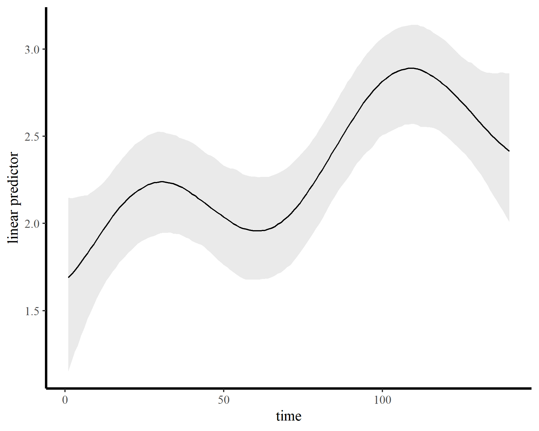
The model fits quickly and encounters few issues. The GP has done an excellent job capturing the nonlinear trend…
plot_links(mod5)
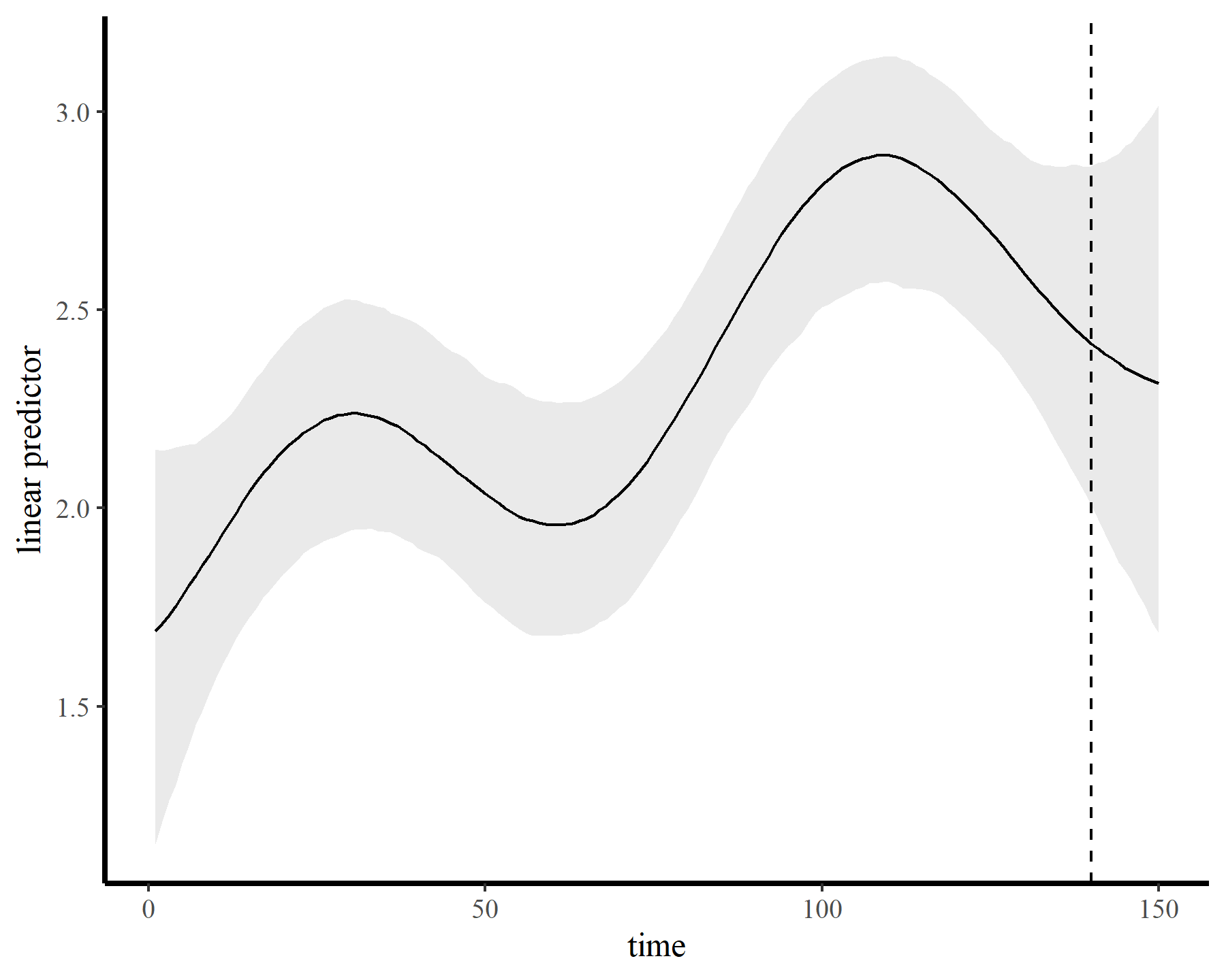
…while also producing sensible extrapolation behaviour:
plot_links(mod5, n_ahead = 10)
Why use Gaussian Processes instead of splines?
“A Gaussian process defines a probability distribution over functions; in other words every sample from a Gaussian Process is an entire function from the covariate space X to the real-valued output space.” (Betancourt; Robust Gaussian Process Modeling)
In many time series analyses, we believe the power of past observations to explain current data is a function of how long ago we observed those past observations. Gaussian Processes use covariance functions (often called ‘kernels’) that allow this to happen by specifying how correlations depend on the difference, in time, between observations. For our purposes we will rely on the squared exponential kernel, which depends on \(\rho\) (often called the length scale parameter) to control how quickly correlations decay as a function of time. The functions also depend on a parameter \(\alpha\), which controls how much the term contributes to the linear predictor. Below we simulate from such a Gaussian Processes to get an idea of the kinds of functional shapes that can be produced as you vary the length scale \(\rho\):
Click here if you would like to see the `R` code used to produce Gaussian Process simulations
# set a seed for reproducibility
set.seed(2222)

# simulate from a fairly large length-scale parameter
rho <- 10

# set the alpha parameter to 1 for all simulations
alpha <- 1

# simulate functions that span 50 time points
times <- 1:50

# generate a sequence of prediction values
draw_seq <- seq(min(times), max(times), length.out = 100)

# construct the temporal covariance matrix
Sigma <- alpha^2 *
  exp(-0.5 * ((outer(draw_seq, draw_seq, "-") / rho) ^ 2)) +
  diag(1e-12, length(draw_seq))

# draw a single realization from the GP distribution
gp_vals <- MASS::mvrnorm(n = 1,
                         mu = rep(0, length(draw_seq)),
                         Sigma = Sigma)

# plot the single GP draw
plot(x = draw_seq, y = gp_vals, type = 'l',
     lwd = 2, col = 'darkred',
     ylab = expression(f(Time)),
     xlab = 'Time', bty = 'l',
     ylim = c(-3.2,3.2),
     main = expression(alpha~'='~1*'; '~rho~'='~10))
# overlay an additional 10 possible functions using different colours
for(i in 1:10){
  draw <- MASS::mvrnorm(n = 1, mu = rep(0, length(draw_seq)),
                        Sigma = Sigma)
  lines(x = draw_seq, y = draw, lwd = 3.5, col = 'white')
  lines(x = draw_seq, y = draw,
        col = sample(c("#DCBCBC",
                       "#C79999",
                       "#B97C7C",
                       "#A25050",
                       "#7C0000"), 1),
        lwd = 2.5)
}
box(bty = 'l', lwd = 2)
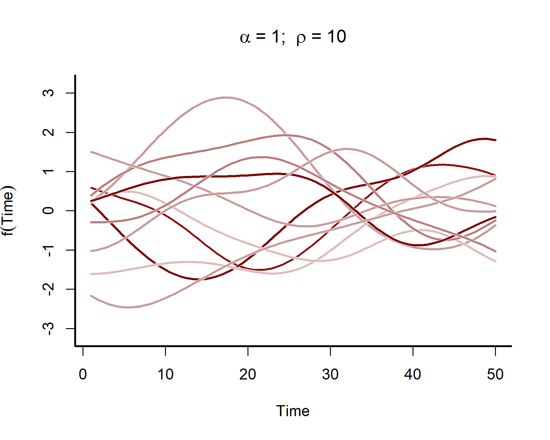
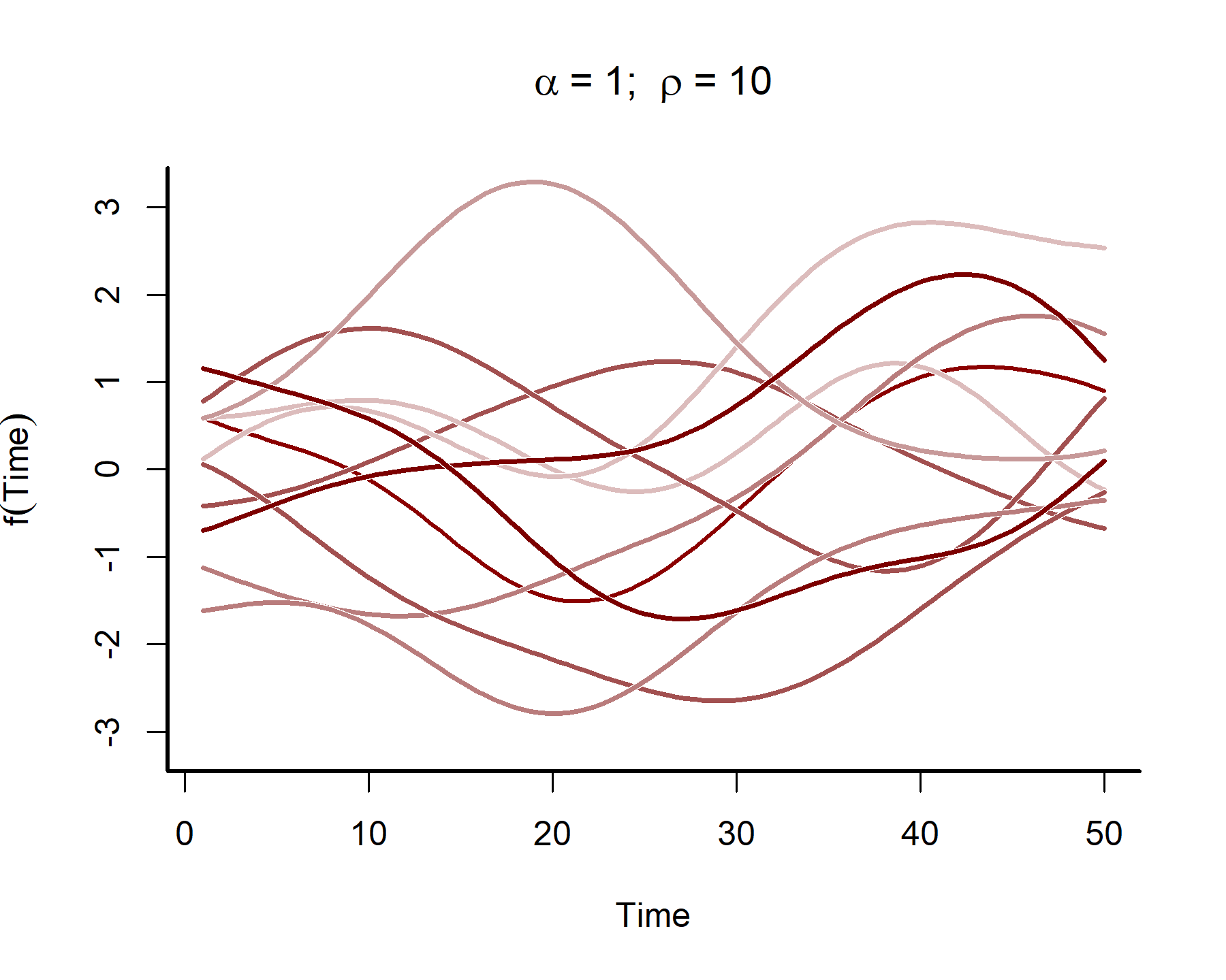
This plot shows that the temporal autocorrelations have a long ‘memory’, i.e. they tend to change slowly over time. In contrast, let’s see what happens when we simulate from a GP with a shorter length scale parameter (the same code as above was used, except the length scale was changed to 4)
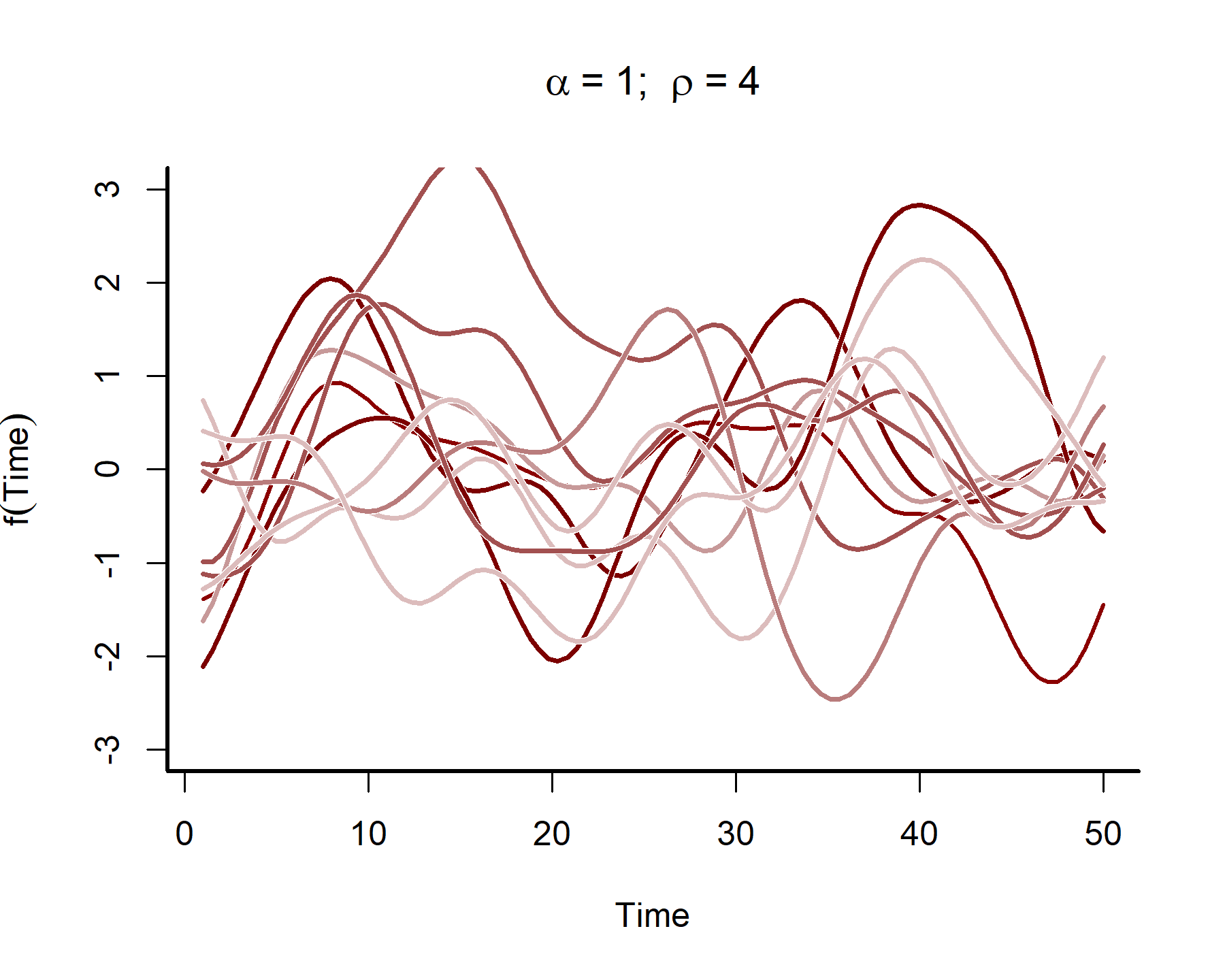
These functions are much ‘wigglier’ and can be useful for capturing temporal dynamics with short-term ‘memory’. A big advantage of Gaussian Processes is that they can easily handle data that are irregularly sampled, much like splines can (and in contrast to autoregressive processes like we’ve been using so far). But although Gaussian Processes may look similar to splines in the functions they return, they are fundamentally different. In particular, a spline has local knowledge, meaning it has no principled way of understanding how the function itself is evolving across time. But a GP directly models how the function changes over time, which means it is better able to generate out-of-sample predictions.
Another big advantage of Gaussian Processes is that their parameters are more directly interpretable than are spline parameters. For instance, the length scale parameter \(\rho\) is related to the stationarity (or stability) of the system. By supplying a prior that pulled this parameter towards larger values, our Bayesian model directly captured our belief that the trend should change smoothly over time (i.e. a long “memory”) and that any unmodelled short-term autocorrelation should be captured by the AR1 process.
By contrast, encoding this sort of information when using splines is incredibly difficult.
Back to interrogating our dynamic model
We can plot how covariance is expected to change over increasing distances in time to understand the long-range “memory” of the Gaussian Process. Those of you that have worked with variograms or semi-variograms before when analysing spatial data will be used to visualizing how semivariance decays over distance. Here we will visualize how covariance decays over time distances (i.e. how far apart in time to we need to be before our estimate from the GP no longer depends on another?). We can define a few helper functions to generate these plots, which will accept posterior estimates of GP parameters from a fitted mvgam object, compute the estimted temporal covariance kernels, calculate posterior quantiles and then plot them:
Click here if you would like to see the `R` function `plot_kernels`, used to plot GP kernels
# Compute the covariance kernel for a given draw
# of GP alpha and rho parameters
quad_kernel = function(rho, alpha, times){
  covs <- alpha ^ 2 *
    exp(-0.5 * ((times / rho) ^ 2))
  return(covs)
}

# Compute kernels for each posterior draw
plot_kernels = function(gp_ests, max_time = 50){
  # set up an empty matrix to store the kernel estimates
  # for each posterior draw
  draw_seq <- seq(0, max_time, length.out = 100)
  kernels <- matrix(NA, nrow = NROW(gp_ests), ncol = 100)

  # use a for-loop to estimate the kernel for each draw using
  # our custom quad_kernel() function
  for(i in 1:NROW(gp_ests)){
    kernels[i,] <- quad_kernel(rho = gp_ests$`rho_gp_trend_time_`[i],
                               alpha = gp_ests$`alpha_gp_trend_time_`[i],
                               times = draw_seq)
  }

  # Calculate posterior empirical quantiles of the kernels
  probs <- c(0.05, 0.2, 0.5, 0.8, 0.95)
  cred <- sapply(1:NCOL(kernels),
                 function(n) quantile(kernels[,n],
                                      probs = probs))

  # Plot the kernel uncertainty estimates
  pred_vals <- draw_seq
  plot(1, xlim = c(0, max_time), ylim = c(0, max(cred)), type = 'n',
       xlab = 'Time difference', ylab = 'Covariance',
       bty = 'L')
  box(bty = 'L', lwd = 2)
  polygon(c(pred_vals, rev(pred_vals)), c(cred[1,], rev(cred[5,])),
          col = "#DCBCBC", border = NA)
  polygon(c(pred_vals, rev(pred_vals)), c(cred[2,], rev(cred[4,])),
          col = "#B97C7C", border = NA)
  lines(pred_vals, cred[3,], col = "#7C0000", lwd = 2.5)
}
Extract posterior estimates of the GP parameters using the as.data.frame function that we’ve been using previously. You can then plot the posterior kernel estimates for model 5 to visualize how temporal error covariance is estimated to change as two time points are further apart. To do this, all we need to supply is the posterior estimates for the GP parameters in the form of a data.frame:
gp_ests <- as.data.frame(mod5, variable = c('rho_gp',
                                            'alpha_gp'),
                         regex = TRUE)
plot_kernels(gp_ests = gp_ests, max_time = 30)
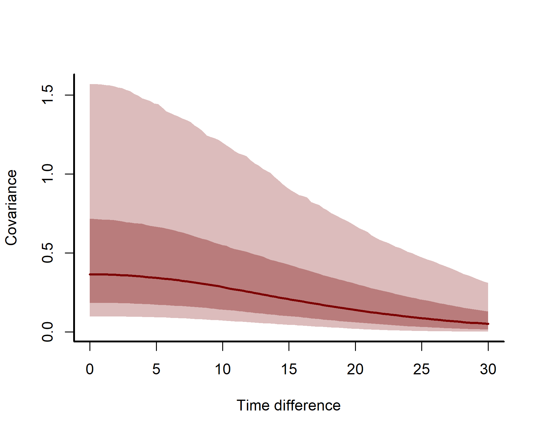 Here we can see how correlations between timepoints decay smoothly as we move further apart in time.
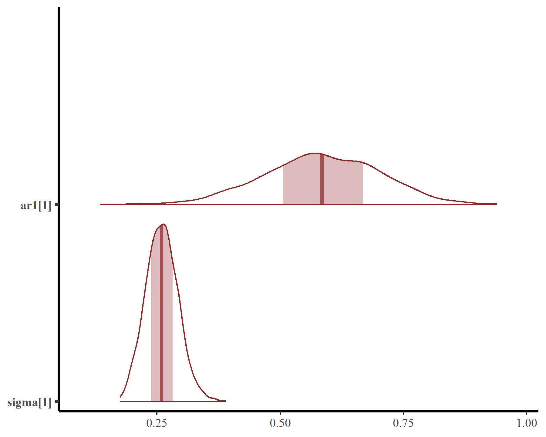
This smooth function is not that complex but works well because we have adequately captured temporal autocorrelation using the latent AR1 process. Estimates of the AR1 parameters come with full uncertainties:
mcmc_plot(mod5, variable = c('ar1', 'sigma'), regex = TRUE, type = 'areas')
Plotting the hindcasts and forecasts won’t work directly with {marginaleffects} as we want to also include the AR1 process. But this is easy to do with {mvgam} functionality
hc <- hindcast(mod5)
plot(hc)
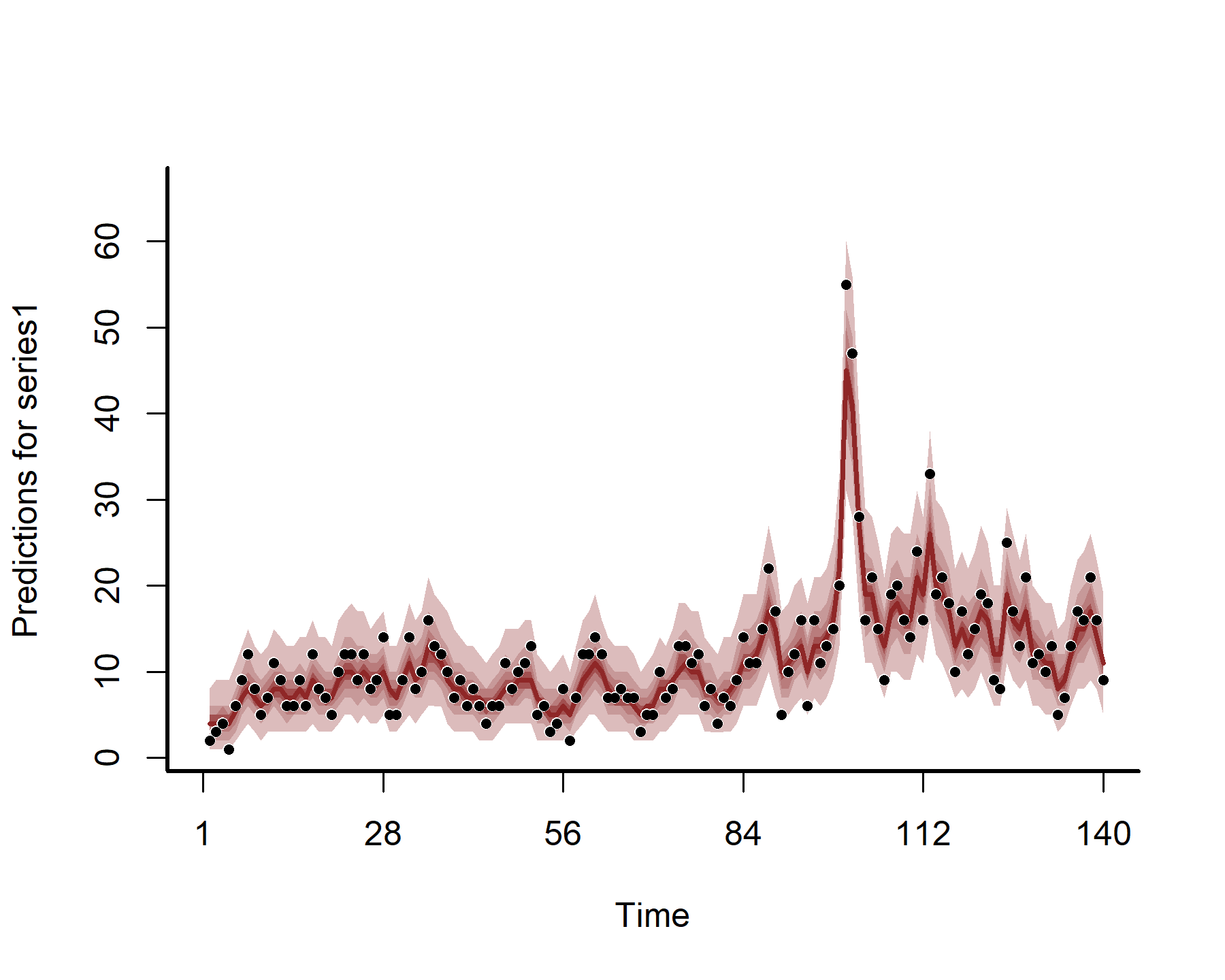
## No non-missing values in test_observations; cannot calculate forecast score
fc <- forecast(mod5, newdata = data.frame(time = (max(dat$time) + 1):(max(dat$time) + 10)))
plot(fc)
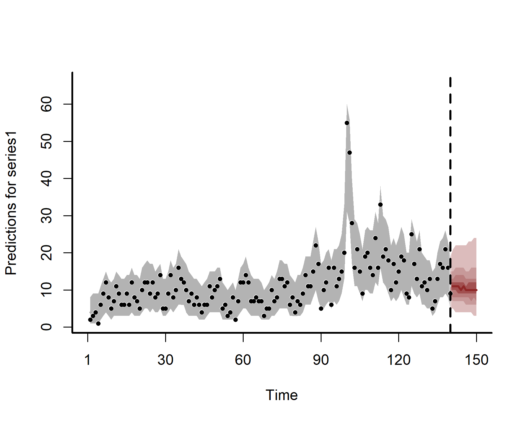
## No non-missing values in test_observations; cannot calculate forecast score
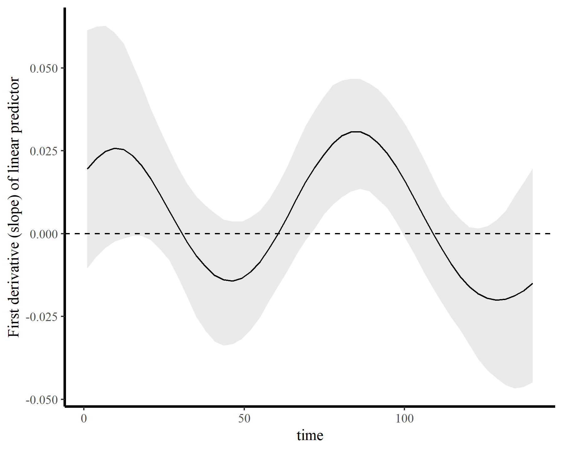
If we wanted to ask targeted questions about the nonlinear trend, we could do this readily. For example, here is the 1st derivative (i.e. the marginal effect) of time, which we can use to ask when the trend was changing most rapidly (i.e. at which time points was the derivative furthest from zero?)
plot_slopes(mod5, variables = 'time', condition = 'time',
            type = 'link') +
  labs(y = 'First derivative (slope) of linear predictor') +
  geom_hline(yintercept = 0, linetype = 'dashed')
There are many more options to capture temporal dynamics and nonlinear effects using dynamic GAMs. For example, my blog post on distributed lag nonlinear models using mgcv and mvgam gives some tips on how to fit lagged covariate effects in GAMs. My research seminar and webinar page also has some good resources and modeling ideas for time series analyses. But we’ll leave those for later posts
Further reading
The following papers and resources offer useful material about modeling time series with Generalized Additive Models
Clark, N. J., Ernest, S. K. M., Senyondo, H., Simonis, J. L., White, E. P., Yennis, G. M., & Karunarathna, K. A. N. K. (2023). Multi-species dependencies improve forecasts of population dynamics in a long-term monitoring study. Biorxiv, doi: https://doi.org/10.32942/X2TS34.
Gasparrini, A. (2014). Modeling exposure–lag–response associations with distributed lag non‐linear models. Statistics in Medicine, 33(5), 881-899.
Pedersen, E. J., Miller, D. L., Simpson, G. L., & Ross, N. (2019). Hierarchical generalized additive models in ecology: an introduction with mgcv. PeerJ, 7, e6876.
Simpson, G. L. (2018). Modelling palaeoecological time series using generalised additive models. Frontiers in Ecology and Evolution, 6, 149.