
Discover more from Gradient Ascent
Houdini & Autoencoders: Escaping the shackles of high-dimensional space
From autoencoders to stable diffusion
Over the next few editions, I'm going to be writing about generative AI techniques. But before we can jump headfirst into Stable Diffusion and the fancy images it produces, we need to look back at some of the fundamentals. That's why I'm covering the humble autoencoder this week. Although it isn't a generative model in the strict sense of the term, learning how it works will help us understand more complicated networks in the coming weeks. Let's dive into the magical world of autoencoders.
This Week on Gradient Ascent:
Understanding autoencoders - The magical basics 🔢
The Prestige of Autoencoders:
"Every great magic trick consists of three parts or acts. The first part is called "The Pledge". The magician shows you something ordinary: a deck of cards, a bird or a man. He shows you this object. Perhaps he asks you to inspect it to see if it is indeed real, unaltered, normal. But of course... it probably isn't. The second act is called "The Turn". The magician takes the ordinary something and makes it do something extraordinary. Now you're looking for the secret... but you won't find it, because of course you're not really looking. You don't really want to know. You want to be fooled. But you wouldn't clap yet. Because making something disappear isn't enough; you have to bring it back. That's why every magic trick has a third act, the hardest part, the part we call "The Prestige"."
- Christopher Priest, The Prestige
I'm a huge Christopher Nolan fan. If you are, too, then you'll probably remember these lines from one of the most underrated movies he's made, "The Prestige". In a Wolverine vs. Batman showdown, Hugh Jackman and Christian Bale feud with each other over a single magic trick. The movie opens with this quote and introduces us to how a magician tricks us into believing that an illusion is real.
Guess what? We have a magic trick or two in the machine learning world too. Let's take a look at the humble autoencoder and how it performs an incredible trick - making data disappear! Let's figure out how it does this.
The Pledge: Introducing the Autoencoder
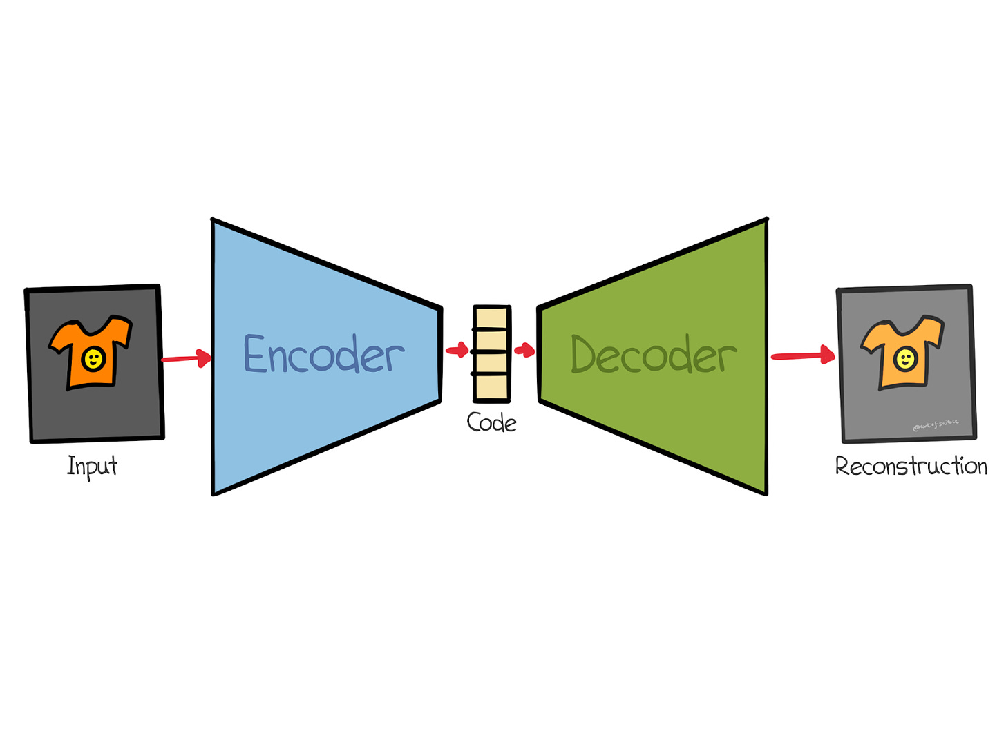
The pledge, or the first part of this magic trick, simply shows what an autoencoder looks like. As you might expect, it looks deceptively simple. It consists of two components, an encoder, and a decoder.
It's an unassuming neural network and, in our example below, consists entirely of linear layers. The input to our autoencoder will be images. Given this input, the autoencoder will make it disappear and magically bring it back.
How does it do so? It learns to represent data in an unsupervised1 manner.
Here's what our autoencoder looks like in code. Note that this architecture is called a stacked (or deep) autoencoder since it consists of several layers stacked together. Also notice that the size of the input gets progressively smaller as it moves through the encoder.
The Turn: Encoding and Compression
The Turn is where the magician takes the ordinary object and makes it do something extraordinary. Our humble autoencoder will now make the input data disappear.
Given an image, the encoder transforms it into a lower-dimensional representation called the latent space. By compressing the input, the autoencoder has to learn the most important features of the input data and can't simply copy over the input.
How does the compression happen? The encoder uses a series of layers that have lower dimensionality than the input. With each successive layer, the input becomes increasingly sparse. Compressing input data is easy, right? Well, how do you recover the original data from the compressed representation?
The Prestige: Decoding and Reconstruction
In the final part of the trick, our autoencoder brings back the original data. The decoder reconstructs the original data from the compressed latent representation. The decoder is typically a mirror image of the encoder and progressively increases the size of the data flowing through it.
Although the reconstruction may not be identical to the original, it will still be very close.
Here's how our autoencoder reconstructed some pictures of clothing items from the Fashion MNIST dataset.
Pretty cool, huh? The real magic of the autoencoder is that it learns how to do this without explicitly being told so.
Behind the Curtain
So far, we've taken for granted that the encoder can compress the input in any way it likes, and the decoder can wave a magic wand and bring the original input back. But, like any magic trick, there's some sleight of hand involved. Let's unpack that next.
Squiggly Deconstruction
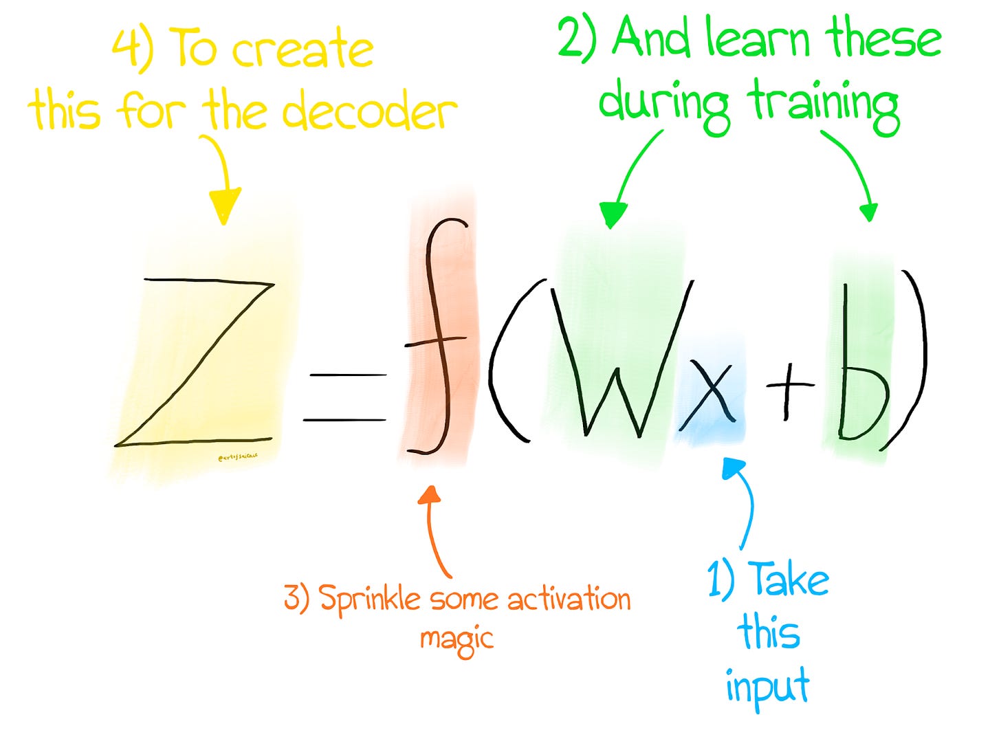
Mathematically, here's how the encoder and decoder are represented.
What are X, Z, and X_hat? They are our input, compressed representation, and reconstruction, respectively. W and b are the weights and biases of the encoder, while W’ and b’ are the weights of the decoder. f and g are activation functions that introduce non-linear magic into the picture. This allows our network to learn complex representations.
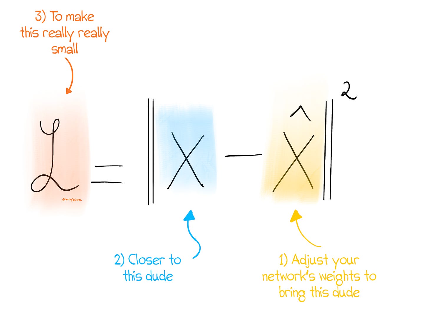
In order for the decoder and encoder to work harmoniously, we have to ensure that X_hat is as close to X as possible. That's where the reconstruction loss comes in. It gives us an idea of how close the reconstructed output is to the input. In this case, we use the mean squared loss (MSE). This computes the difference between the reconstruction and the input and squares it.
Over the course of training, the autoencoder adjusts its weights2 so that this loss becomes smaller and smaller.
Curtain Call: Applications
Autoencoders are pretty nifty and can be used for:
Dimensionality reduction: If you haven't already guessed, autoencoders learn compact representations of data, making them great for reducing the dimensionality of data.
Anomaly Detection: Since autoencoders learn the important features from the input, they can spot abnormalities in data that deviate significantly from normal observations. These weird samples will have a higher reconstruction loss, and thus we can spot them!
Denoising: Autoencoders can be used to remove noise from input data. For example, I added some noise to the images and passed them through the autoencoder. It removed the noise reasonably well.
In the next edition, we'll look at more complex models that overcome the limitations of the simple autoencoder we saw this week. The biggest of these limitations is that a standard autoencoder cannot produce novel samples since it only learns a direct mapping of the input data. How do we solve that? Stay tuned!
P.S.: The code for this week’s article can be found here.
Some would say self-supervised.
Both the encoder and decoder’s weights
Subscribe to Gradient Ascent
Gradient Ascent is your weekly guide to AI, trusted by Silicon Valley's top tech firms and the best academic labs worldwide.









I always enjoy the way you simplify and make the challenging more understandable. This is a great metaphor, well deployed.
nice metaphor!